Coming (swiftly and smoothly) back home after this wonderful and intense week in Banff, I hugged my loved ones,  quickly unpacked, ran a washing machine, and  then sat down to check where and how my reasoning was wrong. To start with, I experimented with a toy example in R:

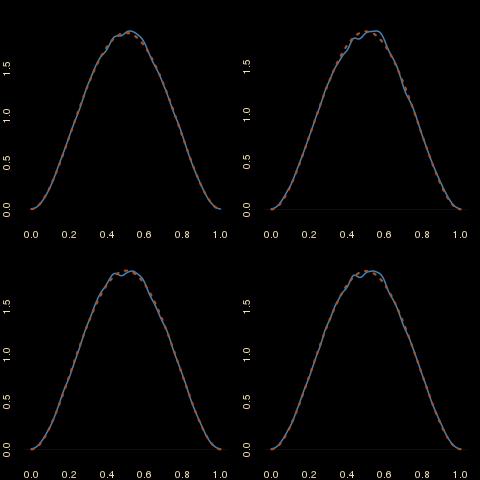
# true target is (x^.7(1-x)^.3) (x^1.3 (1-x)^1.7)
# ie a Beta(3,3) distribution

# samples from partial posteriors
N=10^5
sam1=rbeta(N,1.7,1.3)
sam2=rbeta(N,2.3,2.7)

# first version: product of density estimates
dens1=density(sam1,from=0,to=1)
dens2=density(sam2,from=0,to=1)
prod=dens1$y*dens2$y
# normalising by hand
prod=prod*length(dens1$x)/sum(prod)
plot(dens1$x,prod,type="l",col="steelblue",lwd=2)
curve(dbeta(x,3,3),add=TRUE,col="sienna",lty=3,lwd=2)

# second version: F-S & P's yin+yang sampling
# with weights proportional to the other posterior

subsam1=sam1[sample(1:N,N,prob=dbeta(sam1,2.3,2.7),rep=T)]
plot(density(subsam1,from=0,to=1),col="steelblue",lwd=2)
curve(dbeta(x,3,3),add=T,col="sienna",lty=3,lwd=2)

subsam2=sam2[sample(1:N,N,prob=dbeta(sam2,1.7,1.3),rep=T)]
plot(density(subsam2,from=0,to=1),col="steelblue",lwd=2)
curve(dbeta(x,3,3),add=T,col="sienna",lty=3,lwd=2)

and (of course!) it produced the perfect fits reproduced below. Writing the R code acted as a developing bath as it showed why we could do without the constants!

“Of course”, because the various derivations in the above R code all are clearly independent from the normalising constant: (i) when considering a product of kernel density estimators, as in the first version, this is an approximation of

as well as of

since the constant does not matter. (ii) When considering a sample from m_i and weighting it by the product of the remaining true or estimated m_j‘s, this is a sampling weighting resampling simulation from the density proportional to the product and hence, once again, the constants do not matter. At last, (iii) when mixing the two subsamples, since they both are distributed from the product density, the constants do not matter. As I slowly realised when running this morning (trail-running, not code-runninh!, for the very first time in ten days!), the straight-from-the-box importance sampling version on the mixed samples I considered yesterday (to the point of wondering out loud where did the constants go) is never implemented in the cited papers. Hence, the fact that

is enough to justify handling the target directly as the product of the partial marginals. End of the mystery. Anticlimactic end, sorry…