This is a lecture post for my students in the CUNY MS Data Analytics program. In this series of lectures I discuss mathematical concepts from different perspectives. The goal is to ask questions and challenge standard ways of thinking about what are generally considered basic concepts. I also emphasize using programming to help gain insight into mathematics. Consequently these lectures will not always be as rigorous as they could be.

Numerical integration

A common use of the Monte Carlo method is to perform numerical integration on a function that may be difficult to integrate analytically. This may seem surprising at first, but the intuition is rather straight forward. The key is to think about the problem geometrically and connect this with probability. Let’s take a simple polynomial function, say to illustrate the idea.

Suppose we want to find the integral of this function, but we don’t know how to derive it analytically. All is not lost as we can inscribe the graph into a confined box. Now if we randomly throw grains of rice (ideally points) into the box, the ratio of the number of grains under the curve to the total area of the box will converge to the integral. Intuitively this makes sense because if each point in the box has equal probability of being counted, then it is reasonable that the total probability of the event (of a point being under the curve) is the same as the area under the curve. Indeed, plotting 10,000 random points seems to fill up the box uniformly.

n <- 10000
f <- function(x) x^2
plot(runif(n), runif(n), col='blue', pch=20)
curve(f, 0,1, n=100, col='white', add=TRUE)

Now how do we get from a bunch of points uniformly distributed in a box to an approximation of the integral? To answer this, let’s think about that colloquial phrase “area under the curve”. What this is telling us is that the points under the curve are the important ones. Hence, for a given x value, the y value must be less than the function value at the same point.

ps <- matrix(runif(2*n), ncol=2)
g <- function(x,y) y <= x^2
z <- g(ps[,1], ps[,2])
plot(ps[!z,1], ps[!z,2], col='blue', pch=20)
points(ps[z,1], ps[z,2], col='green', pch=20)
curve(f, 0,1, n=100, col='white', add=TRUE)

The punchline is that the integral is simply the count of all the points under the curve divided by the total number of points, which is the probability that the point lands under the curve.

> length(z[z]) / n
[1] 0.3325

Note that this method is not limited to calculating the integral. It can even be used to approximate irrational numbers like . We’ll explore this scenario a bit later.

Exercises

• Is it okay to use a normal distribution for the Monte Carlo simulation? Explain your answer.
• What happens to the error when the normal distribution is used?

Approximation error and numerical stability

Numerical approximation seems useful, but how do we know whether an approximation is good? To answer this we need to consider the approximation error. Let’s first look at how the approximation changes as we increase the number of points used.

ks <- 1:7
g <- function(k) {
  n <- 10^k
  f <- function(x,y) y <= x^2
  z <- f(runif(n), runif(n))
  length(z[z]) / n
}
a <- sapply(ks,g)

> a
[1] 0.1000000 0.3300000 0.3220000 0.3293000 0.3317400 0.3332160 0.3334584

Judging from this particular realization, it appears that approximation converges, albeit somewhat slowly. Remember that each approximation above took an order of magnitude more samples to produce the result. With 1 million points, the error is about 0.038%. How many points do we need to get to under 0.01%? From Grinstead & Snell we know that the error will be within 95% of the time, which implies that a million trials should achieve a precision of 0.0003162278, or 0.032%. Therefore we need to run 10 million trials to achieve this precision with 95% probability. As a sanity check, in my first attempt I got 0.009071%, which looks good!

When approximations improve as the number of iterations increase, this is known as numerical stability. Plotting out both the theoretical limit and the actual errors shows that with enough terms the two appear to converge.

plot(ks, 1/sqrt(10^ks), type='l')
lines(ks, abs(1/3 - a), col='blue')

Did we answer the question about knowing whether an approximation is good? No, not really. However, attempting to answer this in the abstract is a bit of a fool’s errand. The need for precision is case-specific so there are no fixed rules to follow. It is akin to significance tests that are similarly case-specific. The key is to achieve enough precision that your results don’t create noise when they are used.

Exercises

• What happens when you run the simulation over and over for the same n? Is the result what you expect?

Estimation of

Now it’s time to turn our attention to . As mentioned earlier, it is possible to estimate using a Monte Carlo approach and the same geometric insight. For this situation I use the equation of a circle to define the area. Since the unit circle has area of , a quarter of that will have area . Hence, the end result will need to be multiplied by 4 to get the final approximation.

g <- function(k) {
  n <- 10^k
  f <- function(x,y) sqrt(x^2 + y^2) <= 1
  z <- f(runif(n),runif(n))
  length(z[z]) / n
}
a <- sapply(1:7, g)
> a*4
[1] 3.600000 3.160000 3.100000 3.142800 3.129320 3.142516 3.141445

Similar to the approximation of , the approximation of appears to jump around despite converging to the true value. The amount the value jumps around for a given number of trials is related to the approximation error. In addition to knowing how many iterations must be simulated to get a precise approximation, it is also important to know by how much a given approximation can deviate. We can observe this by running the simulation with the same number of iterations over and over.

trials <- 4 * sapply(rep(6,100), g)
e <- 1/sqrt(10^6)

> mean(trials)
[1] 3.141468
> length(trials[abs(trials - pi)/pi <= e])
[1] 95

Approximation error aside, what is interesting about the Monte Carlo approach is that numerous problems can be solved by transforming a problem into a form compatible with the Monte Carlo approach. Another such class of problems is optimization, which is out of scope for this lecture.

Exercises

• Calculate using a different function f

Simulations

A common use of Monte Carlo methods is for simulation. Rather than approximating a function or number, the goal is to understand a distribution or set of outcomes based on simulating a number of paths through a process. As described in Grinstead & Snell, a simple simulation is tossing a coin multiple times. Here we use a uniform distribution and transform the real-valued output into the set . (The sample function can do this directly, but this is more illustrative.)

r <- runif(1000)
toss <- ifelse(r > .5, 1, -1)
plot(cumsum(toss), type='l')

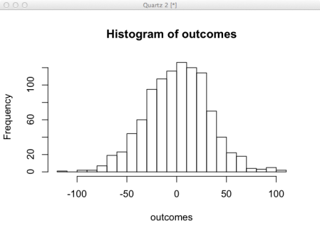
This simulation shows us what happens after randomly tossing a coin 1000 times. It is difficult to glean much information from this, but if we do the same experiment 1000 times, now we can see a good representation of the possible outcomes. Given this set of outcomes it is possible to compute statistics to characterize the properties of the distribution. This is useful when a process doesn’t follow a known distributions.

outcomes <- sapply(1:1000, function(i) sum(ifelse(runif(1000) > .5, 1, -1)))
hist(outcomes)

Exercises

• Change the function to simulate throwing a die instead of tossing a coin
• Plot the histogram. Does this look reasonable to you?