Last year, the good people at is.R() spent December publishing an R advent calendar. This meant that for 24 days, every day, there was an interesting post featuring analysis and some excellent visualizations in R. I think it's an interesting (if very challenging) exercise and I'm going to try to do it myself this year. is.R() has been fairly quiet throughout 2013. I hope that doesn't mean that their effort in December 2012 ruined them.

First, I'll be talking about how this task will be a bit easier thanks to RStudio and knitr. Yihui Xie has some fantastic examples of all the cool stuff you can do with knitr. I'm particularly intrigued by how it can be used to blog. I'll admit that I'm not the biggest fan of the WordPress editor. Moreover, it's counter to the notion of reproducible research. If I'm writing code anyway, why not just upload it directly from RStudio.

Well, you can! William Morris and Carl Boettiger have already figured this out. I had made one half-hearted attempt a few weeks ago, but got hung up on loading images. I've taken a second look at Carl's post and have adopted something very similar to what he has done. FWIW, you can read about image uploading from the master himself here.

First, we'll set options so that the upload function will call a special wrapper to a call to the function RWordPress::uploadFile(). Here, we'll set the options.

opts_knit$set(upload.fun = WrapWordpressUpload, base.url = NULL)
opts_chunk$set(fig.width = 5, fig.height = 5, cache = FALSE)

I set the wrapper function in the calling environment and then knit the R markdown file.

WrapWordpressUpload = function(file) {

    require(RWordPress)

    result = RWordPress::uploadFile(file)

    result$url
}

options(WordPressLogin = c(PirateGrunt = "myPassword"), WordPressURL = "http://PirateGrunt.wordpress.com/xmlrpc.php")

knit2wp("Advent1.Rmd", title = "24 Days of R: Day 1", publish = FALSE, shortcode = TRUE, 
    categories = c("R"))

With that out of the way, we can do some work and have it render neatly in WordPress.

So what do I want to do? Among the things that I'd like to explore is Bayesian analysis. As with most things, I'm a rank novice in this area, but have been playing around a bit. We'll start with my favorite, very easy example: determining whether or not you're dealing with a fair coin. First, we perform a random set of fifty coin tosses with a biased coin.

set.seed(1234)
tosses = 50
p = 0.65
heads = sum(rbinom(tosses, 1, p))

p.hat = heads/tosses

Let's say that we had no prior view as to the fairness of the coin; that is to say, we have a uniform prior. A brute force way to gauge where that prior stands relative to the data, would be to calculate the probability of generating that many heads using a coin with any probability from 0 to 1. Here's how that would work:

test.p = seq(0, 1, length.out = 102)
test.p = test.p[-c(1, 102)]
like = dbinom(heads, tosses, test.p)
best.p = test.p[which(like == max(like))]
plot(test.p, like, ylab = "Likelihood(p)", pch = 19)
abline(v = 0.5, lty = "dotted")
abline(v = p, lty = "solid")
abline(v = best.p, lty = "dashed")

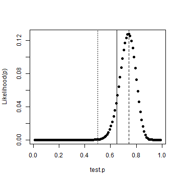
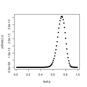
We've also drawn vertial lines for a fair coin, the actual probability and the most likely case given the data. It's clear that we're not dealing with a fair coin. Although instructive, we needn't have done that numerically. I've got a copy of the new Bayesian Data Analysis text by Gelman et al where on page 30, we get a formula for the posterior density.

posterior.p = test.p^heads * (1 - test.p)^(tosses - heads)
plot(test.p, posterior.p, pch = 19, ylab = "p(theta | y)")

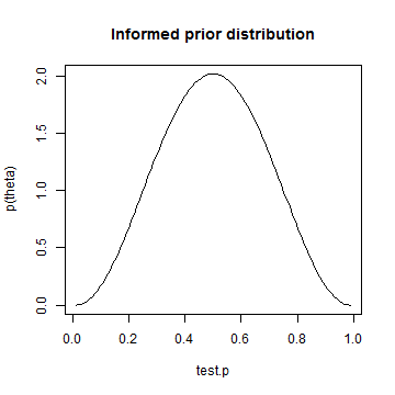
Results are identical, which we would expect. But that's not as interesting as an informed prior. Let's assume that we had reason to believe that the coin was fair, but could allow for some variability. We'll use Jim Albert's beta.select() function to capture the parameters of a beta distribution where one believes that p is centered around 0.5. Those parameters will be applied to the formula near the top of page 35 in Gelman.

library(LearnBayes)
quantile1 = list(p = 0.4, x = 0.45)
quantile2 = list(p = 0.6, x = 0.55)
params = beta.select(quantile1, quantile2)
# My copy of Albert's book is at work. I honestly can't remember which
# parameter is which. I don't think it matters in this case.
alpha = params[1]
beta = params[2]

informed.prior = dbeta(test.p, alpha, beta)
plot(test.p, informed.prior, type = "l", ylab = "p(theta)", main = "Informed prior distribution")

informed.posterior = dbeta(test.p, alpha + heads, beta + tosses - heads)
plot(test.p, informed.posterior, type = "l", ylab = "p(theta|y)", main = "Posterior distribution using informed prior")

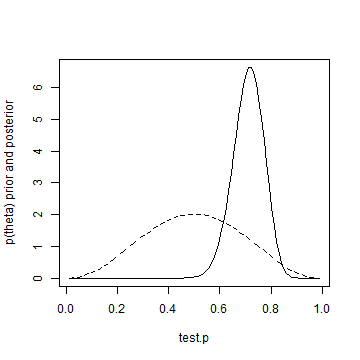
Even with an informed prior, the posterior density moves quite a lot and gets pretty close to the same result as our uniform prior assumption. Just for fun, let's show informed prior and posterior on the same plot.

plot(test.p, informed.posterior, type = "l", ylab = "p(theta) prior and posterior")
lines(test.p, informed.prior, lty = "dashed")

Well, that's it for day one. If you want to test whether or not you're dealing with a fair coin, better flip it 50 times!

Tomorrow, I'm going to draw a few maps. Let's see if I make it 24 straight days.