
From SVG to probability distributions [with R package]
Want to share your content on R-bloggers? click here if you have a blog, or here if you don't.
Hey,
To illustrate generally complex probability density functions on continuous spaces, researchers always use the same examples, for instance mixtures of Gaussian distributions or a banana shaped distribution defined on 
 = \exp\left(-\frac{x^2}{200} - \frac{1}{2}(y+Bx^2-100B)^2\right)")
If we draw a sample from this distribution using MCMC we obtain a [scatter]plot like this one:

Fig. 1: a sample from the very lame banana shaped distribution
Clearly it doesn’t really look like a banana, even if you use yellow to colour the dots like here. Actually it looks more like a boomerang, if anything. I was worried about this for a while, until I came up with a more realistic banana shaped distribution:
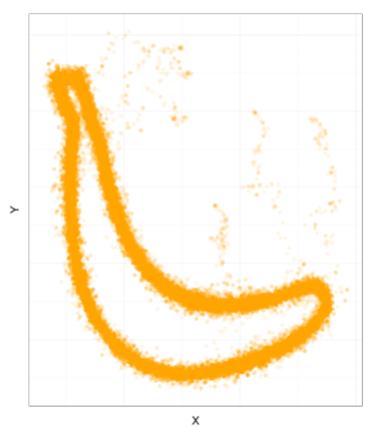
Fig. 2: a sample from the realistic banana shaped distribution
See how the shape is well defined compared to the first figure? And there’s even the little tail, that proves so convenient when we want to peel off the fruit. More generally we might want to create target density functions based on general shapes. For this you can now try RShapeTarget, which you can install directly from R using devtools:
library(devtools)
install_github(repo="RShapeTarget", username="pierrejacob")
The package parses SVG files representing shapes, and creates target densities from them. More precisely, a SVG files contains “paths”, which are sequence of points (for instance the above banana is a single closed path). The associated log density at any point 
 \times d(x, P)")

")


Fig. 3: a sample the “O Canada” probability distribution.
In the package you can get a distribution from a SVG file using the following code:
library(RShapeTarget)
# create target from file
my_shape_target <- create_target_from_shape(my_svg_file_name, lambda =1)
# test the log density function on 25 randomly generated points
my_shape_target$logd(matrix(rnorm(50), ncol = 2), my_shape_target$algo_parameters)
Since characters are just a bunch of paths, you can also define distributions based on words, for instance:

Hodor: Hodor.
which is done as follows (warning you’re only allowed a-z and A-Z, no numbers no space no punctuation for now):
library(RShapeTarget)
word_target <- create_target_from_word("Hodor")
For the words, I defined the target density function as before, except that it’s constant on the letters: so if a point is outside a letter its density is computed based on the distance to the nearest path; if it’s inside a letter it’s just constant, so that the letters are “filled” with some constant density. I thought it’d look better.
Now I’m not worried about the banana shaped distribution any more, but by the fact that the only word I could think of was “Hodor” (with whom you can chat over there).

R-bloggers.com offers daily e-mail updates about R news and tutorials about learning R and many other topics. Click here if you're looking to post or find an R/data-science job.
Want to share your content on R-bloggers? click here if you have a blog, or here if you don't.