Portfolio Trading

Posted on November 12, 2012 by quantsignals in R bloggers | 0 Comments

[This article was first published on quantsignals » R, and kindly contributed to R-bloggers]. (You can report issue about the content on this page here)

Want to share your content on R-bloggers? click here if you have a blog, or here if you don't.

In finance and investing the term portfolio refers to the collection of assets one owns. Compared to just holding a single asset at a time a portfolio has a number of potential benefits. A universe of asset holdings within the portfolio gives a greater access to potentially favorable trends across markets. At the same time the expected risk and return of the overall holding is subject to its specific composition.

A previous post on this blog illustrated a portfolio selection methodology that screens a universe of possible assets. The object there was to find a particular combination that reduces the expected risk-return ratio (sharp-ratio). The assumption there was an underlying buy-and-hold strategy, that once a particular portfolio is selected its composition is hold static until the final position unwound.

This post concerns with dynamic portfolio trading strategies where the portfolio is periodically rebalanced. At prescribed intervals the composition of the portfolio is changed by selling out existing holdings and buying new assets. Typically it is assumed that reallocation does not change the overall portfolio value, with the possible exception of losses due to transaction costs and fees. Another classification concerning this type of strategies is if borrowings are allowed (long-short portfolio) or if all relative portfolio weights are restricted to be positive (long-only portfolio).

Following closely recent publications by Steven Hoi and Bin Li we first set the stage by illustrating fundamental portfolio mechanics and then detailing their passive aggressive mean reversion strategy. We test drive the model in R and test it with 1/2011-11/2012 NYSE and NASDAQ daily stock data.

Portfolio Trading Terminology

Let’s say we want to invest a notional amount of say $\bf P(t=0) = \$ 1,000$ into a portfolio and record each day the total portfolio value $\bf P(t)$ . The portfolio is composed of members with a per share dollar price of $\bf S_i(t)$ . Assuming we hold $\bf \Delta_i(t)$ shares of each component, then the relative portfolio weight for each member is

$\bf b_i(t) = \frac{\Delta^{\$}_i(t)}{P(t)} = \frac{\Delta_i(t) S_i(t)}{P(t)}$ .

The dollar delta $\bf \Delta^{\$}_i(t) = \Delta_i(t) S_i(t)$ expresses the value of each stock holding. Since the aggregated portfolio value is the sum over its components $\bf P(t) = \sum_i \Delta_i(t) S_i(t)$ , the relative portfolio weights are always normalized to $\bf \sum_i b_i(t) = 1$

Buy and Hold

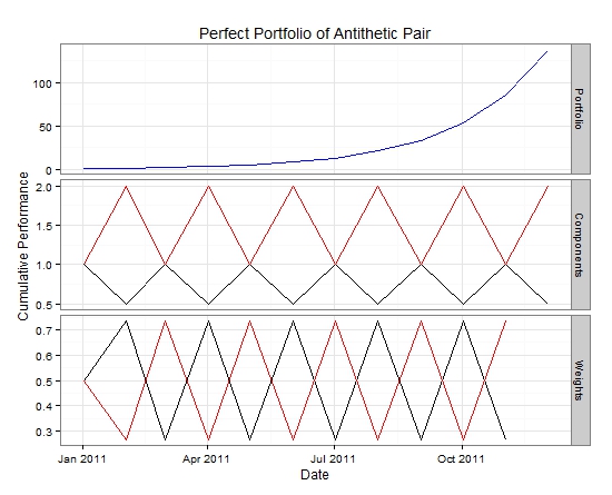
An instructive example is to look at ideal perfectly antithetic pair of artificial price paths. Both assumes assets alternate between a 100% and 50% return. A static portfolio would not experience any growth after a full round trip is completed. The column $\bf x$ shows the individual relative open to close or close to next day’s close returns.

$\bf Day$	$\bf S_1 \atop S_2$	$\bf x_1 \atop x_2$	$\bf b_1 \atop b_2$	$\bf \Delta_1 \atop \Delta_2$	$\bf \Delta^{\$}_1 \atop \Delta^{\$}_2$	$\bf P$
$\bf 1-open$	$\bf \$100 \atop \$100$	$\bf \atop$	$\bf 0.5 \atop 0.5$	$\bf 5 \atop 5$	$\bf \$ 500 \atop \$ 500$	$\bf \$ 1,000$
$\bf 1-close$	$\bf \$ 200 \atop \$ 50$	$\bf 2 \atop 0.5$	$\bf 0.8 \atop 0.2$	$\bf 5 \atop 5$	$\bf \$ 1,000 \atop \$ 250$	$\bf \$ 1,250$
$\bf 2-open$	$\bf \$ 200 \atop \$ 50$	$\bf \atop$	$\bf 0.8 \atop 0.2$	$\bf 5 \atop 5$	$\bf \$ 1,000 \atop \$ 250$	$\bf \$ 1,250$
$\bf 2-close$	$\bf \$ 100 \atop \$ 100$	$\bf 0.5 \atop 2$	$\bf 0.5 \atop 0.5$	$\bf 5 \atop 5$	$\bf \$ 500 \atop \$ 500$	$\bf \$ 1,000$

Dollar Cost Averaging

Dollar cost averaging is a classic strategy that takes advantage of periodic mean reversion. After each close rebalance the portfolio by distributing equal dollar amounts between each component. After the rebalance trades each delta dollar position $\bf \Delta^{\$}(t)$ in the portfolio is the same at the open for each component. Rebalancing itself does not change the total portfolio value. Expressed in terms of the relative portfolio weights $\bf b$ dollar cost averaging is the allocation strategy to rebalance the weight back to the uniform value of the inverse number of components $\bf N$ inside the portfolio.

Dollar cost averaging:
$\bf b_i = 1/N$

$\bf Day$	$\bf S_1 \atop S_2$	$\bf x_1 \atop x_2$	$\bf b_1 \atop b_2$	$\bf \Delta_1 \atop \Delta_2$	$\bf \Delta^{\$}_1 \atop \Delta^{\$}_2$	$\bf P$
$\bf 1-open$	$\bf \$100 \atop \$100$	$\bf \atop$	$\bf 0.5 \atop 0.5$	$\bf 5 \atop 5$	$\bf \$ 500 \atop \$ 500$	$\bf \$ 1,000$
$\bf 1-close$	$\bf \$ 200 \atop \$ 50$	$\bf 2 \atop 0.5$	$\bf 0.8 \atop 0.2$	$\bf 5 \atop 5$	$\bf \$ 1,000 \atop \$ 250$	$\bf \$ 1,250$
$\bf 2-open$	$\bf \$ 200 \atop \$ 50$	$\bf \atop$	$\bf 0.5 \atop 0.5$	$\bf 3.125 \atop 12.5$	$\bf \$ 650 \atop \$ 650$	$\bf \$ 1,250$
$\bf 2-close$	$\bf \$ 100 \atop \$ 100$	$\bf 0.5 \atop 2$	$\bf 0.2 \atop 0.8$	$\bf 3.125 \atop 12.5$	$\bf \$ 312.5 \atop \$ 1,250$	$\bf \$ 1562.5$

Perfect Prediction

With the benefit of perfect foresight its is possible to allocate all weights into the single asset with highest predicted gain.

$\bf Day$	$\bf S_1 \atop S_2$	$\bf x_1 \atop x_2$	$\bf b_1 \atop b_2$	$\bf \Delta_1 \atop \Delta_2$	$\bf \Delta^{\$}_1 \atop \Delta^{\$}_2$	$\bf P$
$\bf 1-open$	$\bf \$100 \atop \$100$	$\bf \atop$	$\bf 1 \atop 0$	$\bf 10 \atop 0$	$\bf \$ 1,000 \atop \$ 0$	$\bf \$ 1,000$
$\bf 1-close$	$\bf \$ 200 \atop \$ 50$	$\bf 2 \atop 0.5$	$\bf 1 \atop 0$	$\bf 10 \atop 0$	$\bf \$ 2,000 \atop \$ 0$	$\bf \$ 2,000$
$\bf 2-open$	$\bf \$ 200 \atop \$ 50$	$\bf \atop$	$\bf 0 \atop 1$	$\bf 0 \atop 40$	$\bf \$ 0 \atop \$ 2,000$	$\bf \$ 2,000$
$\bf 2-close$	$\bf \$ 100 \atop \$ 100$	$\bf 0.5 \atop 2$	$\bf 0 \atop 1$	$\bf 0 \atop 40$	$\bf \$ 0 \atop \$ 4,000$	$\bf \$ 4,000$

Mean Reversion Strategy

The one period portfolio return is given by the product of relative weights and component relative returns as

$\bf L(b,x) = \sum b_i x_i$

The task of the trading strategy is to determine the rebalancing weights $\bf b^{open}(t)$ for the opening position of day $\bf t$ given yesterdays relative returns at the close $\bf x^{close}(t-1)$ .
A forecast of a positive trend would be that today’s returns are a repeat of yesterdays $\bf x^{close}(t) = x^{close}(t-1)$ . In contrast mean reversion would assume that today’s returns are the inverse of yesterdays $\bf x_i^{close}(t) = 1 / x_i^{close}(t-1)$ .

The following strategy consists of determining the weights $\bf b$ such that a positive trend assumption would lead to a loss $\bf L(b^{open}(t),x^{close}(t-1)) = L_0$ with threshold parameter $\bf L_0 \leq 1$ .

Considering returns $\bf \Delta x = x-L_0$ with

$\bf L(b,x) = \sum b_i x_i = L_0$
$\bf = L_0 \sum_i b_i = \sum b_i (x_i - L_0)$
$\bf = \sum b_i \Delta x_i = 0$

Typically the relative performance vector $\bf \Delta x$ consists of a mix of growing and retracting assets. Then we have a balanced number of positive and negative components within the $\bf \Delta x$ vector. The condition that the product $\bf \sum b_i \Delta x_i = 0$ chooses an weight vector that is perpendicular to $\bf \Delta x$ and lies on the unit simplex $\bf \sum b_i =1$ .

Now assume a mean reverting process that consists of a rotation of performances within the asset vector. Graphically the corresponds to a reflection at a $\bf 45$ degree axis. After rotation the angle between the the weight vector and the new performance vectors reduces. This results in an increase of the portfolio return value.

Thus setting for example $\bf L_0 = 1$ generates a flat portfolio in case the performance vector does not change while it increases the portfolio value in the case of an actual mean reversion.

The strategy implicitly assumes a price process that rotates between outperforming and lagging components within the portfolio. This does not include the situation where all stocks are out or underperforming at the same time. The long-only portfolio strategy relies on the ability to be able to reallocate funds between winners and losers.

For the two share example we have

$\bf b_1 = \frac{L_0-x_2}{x_1-x_2}$
$\bf b_2 = \frac{L_0-x_1}{x_2-x_1}$

using $\bf b_1+b_2=1$ and $\bf b_1 x_1 + b_2 x_2 = L_0$

The table below shows the result of computing the portfolio weights at the open of day 2 according to above formulas.

$\bf Day$	$\bf S_1 \atop S_2$	$\bf x_1 \atop x_2$	$\bf b_1 \atop b_2$	$\bf \Delta_1 \atop \Delta_2$	$\bf \Delta^{\$}_1 \atop \Delta^{\$}_2$	$\bf P$
$\bf 1-open$	$\bf \$100 \atop \$100$	$\bf \atop$	$\bf 0.5 \atop 0.5$	$\bf 5 \atop 5$	$\bf \$ 500 \atop \$ 500$	$\bf \$ 1,000$
$\bf 1-close$	$\bf \$ 200 \atop \$ 50$	$\bf 2 \atop 0.5$	$\bf 0.8 \atop 0.2$	$\bf 5 \atop 5$	$\bf \$ 1,000 \atop \$ 250$	$\bf \$ 1,250$
$\bf 2-open$	$\bf \$ 200 \atop \$ 50$	$\bf \atop$	$\bf 0.33 \atop 0.66$	$\bf 2.08 \atop 16.67$	$\bf \$ 416.67 \atop \$ 833.33$	$\bf \$ 1,250$
$\bf 2-close$	$\bf \$ 100 \atop \$ 100$	$\bf 0.5 \atop 2$	$\bf 0.11 \atop 0.89$	$\bf 2.08 \atop 16.67$	$\bf \$ 208.33 \atop \$ 1,666,67$	$\bf \$ 1,875$

With more than two assets the loss condition together with the normalization is not sufficient to uniquely determine the portfolio weights. The additional degrees of freedoms can be used to allow the posing of additional criteria one wishes the strategy to observe. A good choice seems to be requiring that the new portfolio weights are close to the previous selection, as this should minimize rebalance transaction costs.

Minimizing the squared distance between the weights under the normalization and loss constraint leads to the following expression for the new weight

$\bf b(t) = b(t-1) - \tau(t-1) ( x(t-1) - {\bar x}(t-1) )$

as a function of the previous portfolio weights $\bf b(t-1)$ , the return vector $\bf x(t-1)$ and the average return across the portfolio components $\bf {\bar x}(t-1) = \frac{1}{n}\sum_i x_i(t-1)$ .

The control gain $\tau$ is taken as the ratio of the access loss over the return variance

$\bf \tau(t-1) = \frac{ max(0,b(t-1)x(t-1)-L_0 }{ var(x(t-1)) }$

Simulation

This post contains the R code to test the mean reversion strategy. Before running this the function block in the appendix need to be initialized. The following code runs the artificial pair of stocks as a demonstration of the fundamental strategy

# create the antithetic pair of stocks and publish it into the environment
# generate sequence of dates
times <- seq(as.POSIXct(strptime('2011-01-1 16:00:00', '%Y-%m-%d %H:%M:%S')),
                      as.POSIXct(strptime('2011-12-1 16:00:00', '%Y-%m-%d %H:%M:%S')),
                      by="1 months")

# generate and store dummy price series = 200,100,200,100,200 ...
prices.xts <- xts(rep(c(200,100),length(times)/2), order.by=as.POSIXct(times))
stk <- 'STK1'
colnames(prices.xts) <- paste(stk,'.Adjusted',sep="")
assign(x=stk, value=prices.xts, envir=global.env )

# generate and store dummy price series = 100,200,100,200,100 ...
prices.xts <- xts(rep(c(100,200),length(times)/2), order.by=as.POSIXct(times))
stk <- 'STK2'
colnames(prices.xts) <- paste(stk,'.Adjusted',sep="")
assign(x=stk, value=prices.xts, envir=global.env )

# run the strategy and create a plot
strategy(portfolio= c("STK1","STK2"),threshold=.9,doplot=TRUE,title="Artificial Portfolio Example")

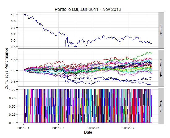
As a benchmark I like always to testing against a portfolio of DJI member stocks using recent 2011 history. The strategy does not do very well for this selection of stocks and recent time frame.

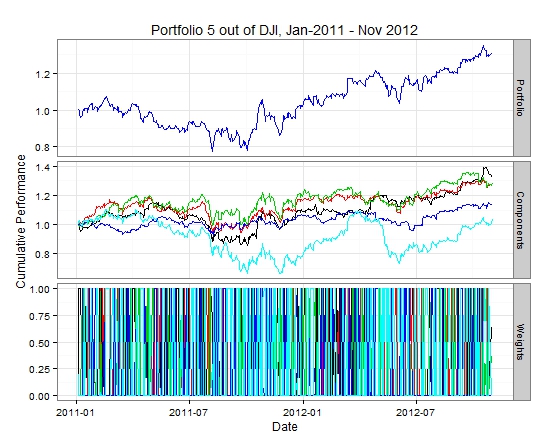
As an enhancement screening stocks by ranking according to their most negative single one-day auto-correlation. The 5 best ranked candidates out of the DJI picked this way are “TRV”,XOM”,”CVX”,PG” and “JPM” .
Rerunning the strategy on the sub portfolio of these five stocks gives a somewhat better performance.

Again, the following code is use to load DJI data from Yahoo and run the strategy

portfolio.DJI <- getIndexComposition('^DJI')
getSymbols(portfolio.DJI,env=global.env)
strategy(portfolio.DJI,.9,TRUE,"2011-01-01::2012-11-01",title="Portfolio DJI, Jan-2011 - Nov 2012")
strategy(c("TRV",XOM","CVX",PG","JPM"),.9,TRUE,"2011-01-01::2012-11-01",title="Portfolio 5 out of DJI, Jan-2011 - Nov 2012")

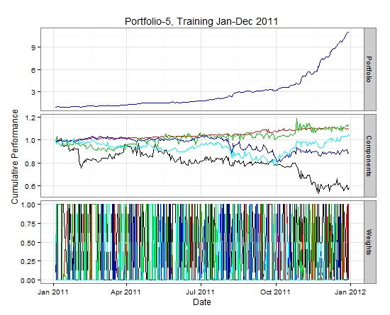
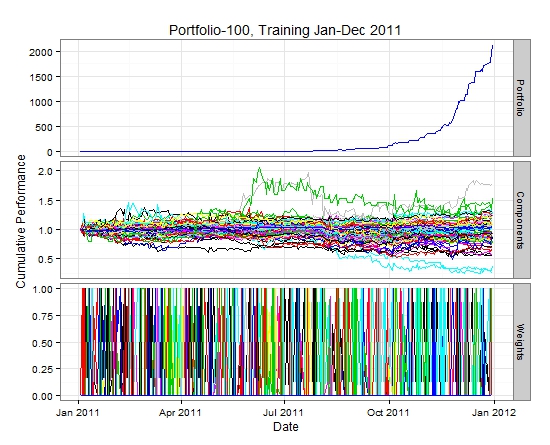
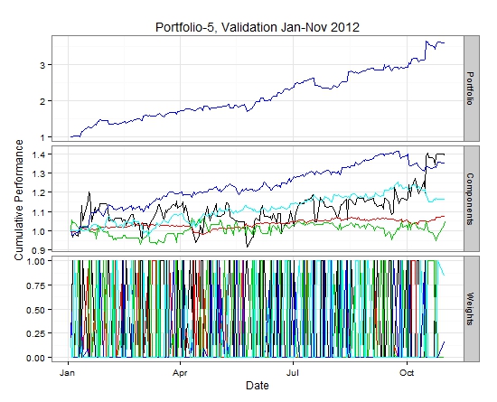
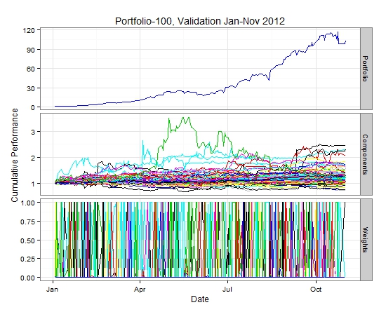
Next a screening a universe of about 5000 NYSE and NASDAQ stocks for those with the best individual auto-correlation within the 2011 time frame. Then running the strategy for 2011 and out of sample in Jan-Nov 2012, with either the 5 or the 100 best names. The constituent portfolio consists of “UBFO”,”TVE”,”GLDC”,”ARI”,”CTBI”.

Discussion

We test drove the passive aggressive trading strategy on recent daily price data. While not doing very well on a mainstream ticker like DJI, pre-screening the stock universe according to a auto-correlation did improve results, even when running the strategy out of sample for the purpose of cross validation. Other extensions, like including a cash asset or allowing for short positions require further investigation.

The strategy has interesting elements, such as minimizing the chance in the portfolio weights and the use of a loss function. It does only directly take the immediate one-period lag into account. For use in other time domains, like high frequency, one could consider having a collection of competing trading agents with a range of time lags that filter out the dominate mean reverting mode.

There are a verity of approaches in the literature that I like to demonstrate as well in the framework of this blog, stay posted.

Appendix: R functions

require(tawny)
require(quantmod)
require(ggplot2)

# global market data environment
global.env <- new.env()

# search anti correlated stocks
# also return daily variance and maximum one day variance
portfolio.screen <- function(portfolio, daterange="")
{
   ac <- matrix()
   for(stk in portfolio)
   {
        p.xts <- Ad(get(stk,global.env)[daterange])
        dr.xts <- dailyReturn(p.xts)
        dr.maxvar <- max( (dr.xts-mean(dr.xts) )^2)
        dr.var <- coredata(var(dr.xts))
        dr.var.ratio <- dr.maxvar/(dr.var)
        dr.ac <-  coredata( acf(dr.xts)$acf[1:5] )
        dr.ac.res <- c(stk, dr.var.ratio, dr.maxvar, dr.var, dr.ac)

       if(length(ac)==1)
       {
          ac <- dr.ac.res
       }
       else
       {   
          ac <- rbind(ac, dr.ac.res)
       }
}
# sort by decreasing auto-correlations
ac_sort <- (ac[order(as.numeric(ac[,6]),decreasing='FALSE'),])
# return sorted matrix of stocks and correlations
ac_sort
}

#############################################################################
# portfolio weight vector b
# price relative return vector x
# threshold parameter e, usually e <= 1 for

# returns intrinsic value of call on portfolio return with strike e
strategy.loss <- function(b, x, e)
{
    max(b%*%x-e,0)
}

strategy.gearing <- function(b, x, e)
{
    loss <- strategy.loss(b,x,e)
    varx <- var(x)
    if(varx>0) { -loss/varx }
    else { 0}
}

# return a vector w so that w is close to v
# by minimizing the distance (w-v)^2
# with the condition that w is on the simplex
# sum(w)=1
strategy.simplex <- function(v,z)
{   
    # initialize projection to zero
    w <- rep(0, length(v) )
    # Sort v into u in descending order

    idx <- order(v,decreasing=TRUE)
    u <- v[idx]

    #index of number of non zero elements in w
    rho <-max(index(u)[index(u)*u  >= cumsum(u) -z])
    if(rho>0)
    {
       theta <-(sum(u[1:rho])-z)/rho
       w[idx[1:rho]] <- v[idx[1:rho]] - theta;
    }
 w
}

strategy.rebalance <- function(b,x,e)
{
    dbdx <- strategy.gearing <- strategy.gearing(b, x, e)
    b_new <- b + dbdx*(x-mean(x))
    b_new <- strategy.simplex(b_new,1)
}

############################################
###################################
# Simulate the portfolio trading strategy
# Arguments:
# portfolio : portfolio of stocks f
# threshold: mean reversion loss parameter ( should be in the order but smaller than 1)
# doplot: create an optional plot
# daterange: range of dates to test
#
# returns the accumulated gain of the strategy
#
strategy <- function(portfolio, threshold=1, doplot=FALSE,daterange="",title="" )
{
   portfolio.prices.xts <- xts()
   # raw portfolio components price time series
   for( stk in portfolio)
   {
       portfolio.prices.xts <- cbind(portfolio.prices.xts, Ad(get(stk,envir = global.env)[daterange]))
   }
   # downfill missing closing prices (last observation carried forward)

   portfolio.prices.xts <- na.locf(portfolio.prices.xts)
   
    # not backfill missing history backwards, for example for IPO assets that did
    # not exist, we set these to the constant initial 'IPO' price , resembling a cash asset
    
    portfolio.prices.xts <- na.locf(portfolio.prices.xts,fromLast=TRUE)
    times <- index(portfolio.prices.xts) 
    nprices <- NROW(portfolio.prices.xts)

     # relative prices S(t)/S(t-1)
     portfolio.price.relatives.xts <- (portfolio.prices.xts/lag(portfolio.prices.xts,1))[2:nprices,]

     # initialize portfolio weights time series
     portfolio.weights.xts <- xts(matrix(0,ncol=length(portfolio),nrow=nprices-1),
                                           order.by=as.POSIXct(times[2:nprices]))

     colnames(portfolio.weights.xts) = portfolio

     # initialize strategy with equal weights
     portfolio.weights.xts[1,] = rep(1/length(portfolio),length(portfolio))

     # run strategy:
     for( i in 1:(nprices-2))
     {
        #portfolio weights at opening of the day
        b_open <- portfolio.weights.xts[i,]

        #price relative return at close x = S(t)/S(t-1)
        x_close <- portfolio.price.relatives.xts[i,]

       # compute end of day rebalancing portfolio with strategy
       b_new <-  strategy.rebalance(as.vector(b_open),as.vector(x_close),threshold)

       # assign portfolio composition for next day opening
       portfolio.weights.xts[i+1,] <- b_new
      }

   #aggregate portfolio returns

    portfolio.total.relatives.xts <- xts( rowSums(portfolio.weights.xts * portfolio.price.relatives.xts), order.by=as.POSIXct(times[2:nprices]))
     portfolio.cum.return.xts <- cumprod( portfolio.total.relatives.xts)

    # cummulative wealth gained by portfolio

    if(doplot==TRUE)
    {
      Times <- times
      df<-data.frame(Date=Times,

      Performance=c(1,coredata(portfolio.cum.return.xts)), pane='Portfolio')
      myplot <- ggplot()+theme_bw()+
      facet_grid (pane ~ ., scale='free_y')+
      labs(title=title) +
      ylab("Cumulative Performance ") +
      geom_line(data = df,  aes(x = Date, y = Performance), color="blue")

      for(i in 1:length(portfolio))
      {
        df1<-data.frame(Date=Times, Performance=c(1,coredata(cumprod(portfolio.price.relatives.xts[,i] ) ) ),pane='Components')
        names(df1)[2] <- "Performance"
        myplot <- myplot +
        geom_line(data = df1, aes_string(x = "Date", y = "Performance"),color=i)

        df3<-data.frame(Date=Times, Performance=c(1,coredata(cumprod(portfolio.price.relatives.xts[,i] ) ) ), pane='Components')
         names(df1)[2] <- "Performance"
         myplot <- myplot +
         geom_line(data = df1, aes_string(x = "Date", y = "Performance"),color=i)

          df2<-data.frame(Date=Times[1:NROW(Times)-1],
          Weights=coredata(portfolio.weights.xts[,i]) , pane='Weights')

          names(df2)[2] <- "Weights"

           myplot <- myplot + geom_line(data = df2, aes_string(x = "Date", y = "Weights"),color=i)
         }
     print(myplot)
} # end of plotting

# return performance
last(portfolio.cum.return.xts)
}

To leave a comment for the author, please follow the link and comment on their blog: quantsignals » R.

R-bloggers.com offers daily e-mail updates about R news and tutorials about learning R and many other topics. Click here if you're looking to post or find an R/data-science job.

Want to share your content on R-bloggers? click here if you have a blog, or here if you don't.

R-bloggers

R news and tutorials contributed by hundreds of R bloggers

Portfolio Trading

Portfolio Trading Terminology

Buy and Hold

Dollar Cost Averaging

Perfect Prediction

Mean Reversion Strategy

Simulation

Discussion

Appendix: R functions

Related

Portfolio Trading Terminology

Buy and Hold

Dollar Cost Averaging

Perfect Prediction

Mean Reversion Strategy

Simulation

Discussion

Appendix: R functions

Related

Never miss an update! Subscribe to R-bloggers to receive e-mails with the latest R posts. (You will not see this message again.)

Never miss an update!
Subscribe to R-bloggers to receive
e-mails with the latest R posts.
(You will not see this message again.)