A number of years ago, someone asked me “why does my company need actuaries to fit curves, once I have the mean and standard deviation of my losses, isn’t that enough?” I explained to him that not every distribution is completely determined by its mean and standard deviation (as the normal and lognormal are), and as at that point, I did not have “R” installed on my laptop, I demonstrated it to him in Excel. Having wanted to start blogging about “R”, even ever so infrequently, I figured I’d toss together a little code to demonstrate.

The example I gave was to compare a gamma and a pareto distribution, each of which has mean 10,000 and a CV of 150% (making the standard deviation 15,000). I will spare all of you the algebra, but suffice to say, that using the Klugman-Panjer-Wilmot parameterization (which is used by most casualty actuaries in the past 20 years or so) the parameters of the gamma would be theta (R’s scale) = 22500 and alpha (R’s shape) = 4/9. The equivalent pareto would have theta (R’s scale) = 26000 and alpha (R’s shape) = 3.6.

Graphing the two (and Hadley, please forgive me for using default R’ plotting, I left my ggplot book in the office; mea culpa) you can easily see how the distributions are rather different.

 

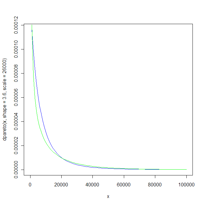
To make things easier for me, I used the actuar  package to do the graphing:

library(actuar)
curve(dpareto(x, shape=3.6, scale=26000), from=0, to=100000, col="blue")
curve(dgamma(x, shape=4/9, scale=22500), from=0, to=100000, add=TRUE, col="green")

Obviously, the tails of the distributions, and thus the survival function at a given loss size, is different for the two, notwithstanding their sharing identical first two moments. So, this was just a brief but effective visualization as to how the first two moments do not contain all the information needed to find a “best fit,” and why we like to use distributional fitting methods (maximum likelihood, maximum spacing, various minimum distance metrics like Cramer-von Mises, etc.) to get a better understanding of the potential underlying loss processes.