
Testing Assumption Testing
Want to share your content on R-bloggers? click here if you have a blog, or here if you don't.
I’ve been doing a lot of linear modeling this year. That’s not much different than any ordinary year, but now I’m doing it in R. I had spent a bit of time in recent years trying to look at loss reserving as a multivariate regression. Excel is happy to do that, but testing various predictor variables and applying the methodology to many data sets required significant VBA to move the data from place to place. Further, all of the really cool diagnostics aren’t part of Excel’s standard toolkit, so I rarely used them. F tests and t tests were about as sophisticated as it got.
That’s a shame, because if you’re not testing the underlying assumptions of your model, your model might very well be rubbish. Earlier this year, while trolling the actuarial literature for wisdom about model diagnostics, I ran across some papers which discussed testing the underlying assumptions of a model. Ordinary least squares regression presumes a multivariate, homoskedastic normal. Any non-life actuary, when asked, will tell you that their data doesn’t adhere to those assumptions. OK. Have they been tested?
Just for kicks one day, I ran a Monte Carlo simulation to see which normalcy test functioned best under a number of different circumstances. I generated 10,000 trials of 10, 50, 100 and 1000 sample points. I did this for normally and lognormally distributed variables. (Actually, I did this for uniform and exponential variables as well, but haven’t put them up here.)
I needn’t remind anyone that there are two types of errors that a test can make. It can reject a hypothesis that it shouldn’t and it can fail to reject a hypothesis that it should. The first type of error is controllable via the significance level of the test. The second is a bit murkier. If I generate a random sample from a lognormal distribution, the probability of a type I error is zero. The hypothesis should always be rejected, so there’s no danger of “accidentally” rejecting it. For the type II error, there’s really no easy way of knowing. So, let’s generate a large pile of random numbers and see what happens.
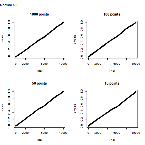
Samples generated from a normal distribution behave as expected. Below is the distribution of Anderson-Darling p values for 10,000 trials of one thousand, one hundred, fifty and ten sample points. It’s more or less a straight line. This means that the probability of a type I error is about equal to the significance level. The probability of a type II error is, of course, zero.
Let’s see the same results for a lognormal distribution. Again, the probability of a type I error is zero. For 1,000 sample points, the chance of a type II error is remote, roughly one chance in 10,000. With smaller samples, that chance increases, as we would expect.

So that’s how well Anderson Darling performs. How about the other tests?
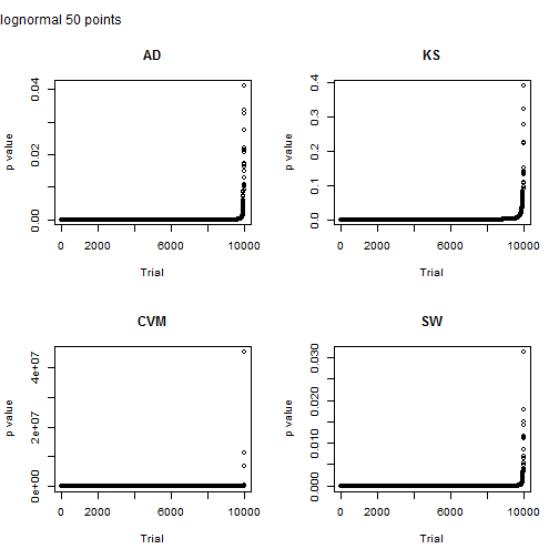
Here I look at a sample size of 50 points. Note that scale on the y axis for the Cramer von-Mises test. Something clearly went nuts for three points and they have a p value greater than one. The p value for the other tests is less than the typical 5% for the other tests, but Shapiro-Wilkes is just a shade lower.
Very big caveat: I’m not adjusting the variance. High variance will undoubtedly affect the strength of the various tests and is an important consideration. I may get around to that at some point.
So why is this relevant to actuaries? Two reasons. One, most applications of traditional loss reserving techniques are de facto linear models. The calibration of the model parameters and the variance around the estimates rely on assumptions about the error structure. Those assumptions ought to be tested. Two, the way that loss reserving data is structured means that you’ve usually only got around 10 sample points. So, you’re more likely than not to run into situations where you hit a type II error. In other words, you’ll not reject your model even though you ought to.
By the way, if you want a fantastic overview of the various apply functions, look no further than here: http://nsaunders.wordpress.com/2010/08/20/a-brief-introduction-to-apply-in-r/
Shapiro-Wilkes will likely be my knee jerk test of normalcy going forward. As always, individual mileage may vary and for heaven’s sake don’t use a tool unless you know how it’s meant to be used. So, as usual, one answer will lead to a few more questions and a bit more homework.
And now some code:
SampleTests = function(sample)
{
  AD = ad.test(sample)
  CVM = cvm.test(sample)
  KS = lillie.test(sample)
  SW = shapiro.test(sample)
  aVector = c(AD$statistic
              , AD$p.value
              , CVM$statistic
              , CVM$p.value
              , KS$statistic
              , KS$p.value
              , SW$statistic
              , SW$p.value)

  return (aVector)
}

GetTrials = function(sample)
{
  testResults = apply(sample, 2, SampleTests)
  df = t(testResults)
  df = as.data.frame(df)
  colnames(df) = c("AD.stat"
                  , "AD.pVal"
                  , "CVM.stat"
                  , "CVM.pVal"
                  , "KS.stat"
                  , "KS.pVal"
                  , "SW.stat"
                  , "SW.pVal")
  return (df)
}

trials = 10000
sampleSize = 1000

sample.normal = replicate(trials, rnorm(sampleSize, mean=0, sd=1))
sample.lognormal = replicate(trials, rlnorm(sampleSize, meanlog=0, sdlog = 1))

df1000.normal = GetTrials(sample.normal)
df100.normal = GetTrials(sample.normal[1:100,])
df50.normal = GetTrials(sample.normal[1:50,])
df10.normal = GetTrials(sample.normal[1:10,])

df1000.lognormal = GetTrials(sample.lognormal)
df100.lognormal = GetTrials(sample.lognormal[1:100,])
df50.lognormal = GetTrials(sample.lognormal[1:50,])
df10.lognormal = GetTrials(sample.lognormal[1:10,])
par(mfrow=c(2,2), oma=c(0,0,2,0))
plot(sort(df1000.normal$AD.pVal), main = "1000 points", ylab = "p value", xlab = "Trial")
plot(sort(df100.normal$AD.pVal), main = "100 points", ylab = "p value", xlab = "Trial")
plot(sort(df50.normal$AD.pVal), main = "50 points", ylab = "p value", xlab = "Trial")
plot(sort(df10.normal$AD.pVal), main = "10 points", ylab = "p value", xlab = "Trial")
mtext("Normal AD", side=3, outer=TRUE, line=0, adj=0)

plot(sort(df50.lognormal$AD.pVal), main = "AD", ylab = "p value", xlab = "Trial")
plot(sort(df50.lognormal$KS.pVal), main = "KS", ylab = "p value", xlab = "Trial")
plot(sort(df50.lognormal$CVM.pVal), main = "CVM", ylab = "p value", xlab = "Trial")
plot(sort(df50.lognormal$SW.pVal), main = "SW", ylab = "p value", xlab = "Trial")
mtext("lognormal 50 points", side=3, outer=TRUE, line=0, adj=0)

R-bloggers.com offers daily e-mail updates about R news and tutorials about learning R and many other topics. Click here if you're looking to post or find an R/data-science job.
Want to share your content on R-bloggers? click here if you have a blog, or here if you don't.