
Taking a closer look at Quantum gates and their operations
Want to share your content on R-bloggers? click here if you have a blog, or here if you don't.
This post is a continuation of my earlier post ‘Exploring Quantum gate operations with QCSimulator’. Here I take a closer look at more quantum gates and their operations, besides implementing these new gates in my Quantum Computing simulator, the QCSimulator in R.
Disclaimer: This article represents the author’s viewpoint only and doesn’t necessarily represent IBM’s positions, strategies or opinions
In quantum circuits, gates are unitary matrices which operate on 1,2 or 3 qubit systems which are represented as below
1 qubit
|0> = 
2 qubits
|0> 
|0>
|1>
|1>
3 qubits
|0>
|0>
|0>
…
…
|1>
Hence single qubit is represented as 2 x 1 matrix, 2 qubit as 4 x 1 matrix and 3 qubit as 8 x 1 matrix


1) Composing Quantum gates in series
When quantum gates are connected in a series. The overall effect of the these quantum gates in series is obtained my taking the dot product of the unitary gates in reverse. For e.g.

In the following picture the effect of the quantum gates A,B,C is the dot product of the gates taken reverse order
result = C . B . A
This overall action of the 3 quantum gates can be represented by a single ‘transfer’ matrix which is the dot product of the gates

If we had a Pauli X followed by a Hadamard gate the combined effect of these gates on the inputs can be deduced by constructing a truth table
| Input | Pauli X – Output A’ | Hadamard – Output B |
| |0> | |1> | 1/√2(|0> – |1>) |
| |1> | |0> | 1/√2(|0> + |1>) |
Or
|0> -> 1/√2(|0> – |1>)
|1> -> 1/√2(|0> + |1>)
which is

Therefore the ‘transfer’ matrix can be written as
T = 1/√2


2)Quantum gates in parallel
When quantum gates are in parallel then the composite effect of the gates can be obtained by taking the tensor product of the quantum gates.
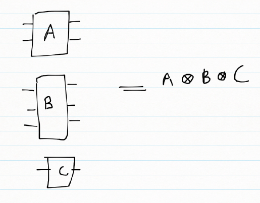
If we consider the combined action of a Pauli X gate and a Hadamard gate in parallel

| A | B | A’ | B’ |
| |0> | |0> | |1> | 1/√2(|0> + |1>) |
| |0> | |1> | |1> | 1/√2(|0> – |1>) |
| |1> | |0> | |0> | 1/√2(|0> + |1>) |
| |1> | |1> | |0> | 1/√2(|0> – |1>) |
Or
|00> => |1>
|01> => |1>
|10> => |0>
|11> => |0>
|00> = 
|01> = 
|10> = 
|11> = 


Here are more Quantum gates
a) Rotation gate

b) Toffoli gate
The Toffoli gate flips the 3rd qubit if the 1st and 2nd qubit are |1>
| Toffoli gate | |
| Input | Output |
| |000> | |000> |
| |001> | |001> |
| |010> | |010> |
| |011> | |011> |
| |100> | |100> |
| |101> | |101> |
| |110> | |111> |
| |111> | |110> |
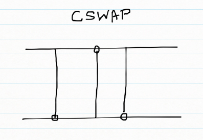
c) Fredkin gate
The Fredkin gate swaps the 2nd and 3rd qubits if the 1st qubit is |1>
| Fredkin gate | |
| Input | Output |
| |000> | |000> |
| |001> | |001> |
| |010> | |010> |
| |011> | |011> |
| |100> | |100> |
| |101> | |110> |
| |110> | |101> |
| |111> | |111> |
d) Controlled U gate
A controlled U gate can be represented as
controlled U = 
where U =

e) Controlled Pauli gates
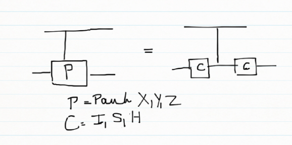
Controlled Pauli gates are created based on the following identities. The CNOT gate is a controlled Pauli X gate where controlled U is a Pauli X gate and matches the CNOT unitary matrix. Pauli gates can be constructed using
a) H x X x H = Z &
H x H = I
b) S x X x S1
S x S1 = I
the controlled Pauli X, Y , Z are contructed using the CNOT for the controlled X in the above identities
In general a controlled Pauli gate can be created as below
f) CPauliX
Here C is the 2 x2 Identity matrix. Simulating this in my QCSimulator
CPauliX <- function(q){

I=matrix(c(1,0,0,1),nrow=2,ncol=2)

# Compute 1st composite

a = TensorProd(I,I)

b = CNOT2_01(a)

# Compute 1st composite

c = TensorProd(I,I)

#Take dot product

d = DotProduct(c,b)

#Take dot product with qubit

e = DotProduct(d,q)

e

}
Implementing the above with I, S, H gives Pauli X, Y and Z as seen below
library(QCSimulator)
I4=matrix(c(1,0,0,0,
            0,1,0,0,
            0,0,1,0,
            0,0,0,1),nrow=4,ncol=4)

#Controlled Pauli X
CPauliX(I4)
##      [,1] [,2] [,3] [,4]
## [1,]    1    0    0    0
## [2,]    0    1    0    0
## [3,]    0    0    0    1
## [4,]    0    0    1    0
#Controlled Pauli Y
CPauliY(I4)
##      [,1] [,2] [,3] [,4]
## [1,] 1+0i 0+0i 0+0i 0+0i
## [2,] 0+0i 1+0i 0+0i 0+0i
## [3,] 0+0i 0+0i 0+0i 0-1i
## [4,] 0+0i 0+0i 0+1i 0+0i
#Controlled Pauli Z
CPauliZ(I4)
##      [,1] [,2] [,3] [,4]
## [1,]    1    0    0    0
## [2,]    0    1    0    0
## [3,]    0    0    1    0
## [4,]    0    0    0   -1
g) CSWAP gate
q00=matrix(c(1,0,0,0),nrow=4,ncol=1)
q01=matrix(c(0,1,0,0),nrow=4,ncol=1)
q10=matrix(c(0,0,1,0),nrow=4,ncol=1)
q11=matrix(c(0,0,0,1),nrow=4,ncol=1)
CSWAP(q00)
##      [,1]
## [1,]    1
## [2,]    0
## [3,]    0
## [4,]    0
#Swap qubits
CSWAP(q01)
##      [,1]
## [1,]    0
## [2,]    0
## [3,]    1
## [4,]    0
#Swap qubits
CSWAP(q10)
##      [,1]
## [1,]    0
## [2,]    1
## [3,]    0
## [4,]    0
CSWAP(q11)
##      [,1]
## [1,]    0
## [2,]    0
## [3,]    0
## [4,]    1
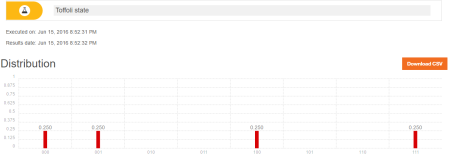
h) Toffoli state
The Toffoli state creates a 3 qubit entangled state 1/2(|000> + |001> + |100> + |111>)

Simulating the Toffoli state in IBM Quantum Experience we get
h) Implementation of Toffoli state in QCSimulator
#ToffoliState <- function(q)
    # Computation of the Toffoli State
    H=1/sqrt(2) * matrix(c(1,1,1,-1),nrow=2,ncol=2)
    I=matrix(c(1,0,0,1),nrow=2,ncol=2)

    # 1st composite
    # H x H x H
    a = TensorProd(TensorProd(H,H),H)
    # 1st CNOT
    a1= CNOT3_12(a)

    # 2nd composite
    # I x I x T1Gate
    b = TensorProd(TensorProd(I,I),T1Gate(I))
    b1 = DotProduct(b,a1)
    c = CNOT3_02(b1)

    # 3rd composite
    # I x I x TGate
    d = TensorProd(TensorProd(I,I),TGate(I))
    d1 = DotProduct(d,c)
    e = CNOT3_12(d1)

    # 4th composite
    # I x I x T1Gate
    f = TensorProd(TensorProd(I,I),T1Gate(I))
    f1 = DotProduct(f,e)
    g = CNOT3_02(f1)

    #5th composite
    # I x T x T
    h = TensorProd(TensorProd(I,TGate(I)),TGate(I))
    h1 = DotProduct(h,g)
    i = CNOT3_12(h1)

    #6th composite
    # I x H x H
    j = TensorProd(TensorProd(I,Hadamard(I)),Hadamard(I))
    j1 = DotProduct(j,i)
    k = CNOT3_12(j1)

    # 7th composite
    # I x H x H
    l = TensorProd(TensorProd(I,Hadamard(I)),Hadamard(I))
    l1 = DotProduct(l,k)
    m = CNOT3_12(l1)
    n = CNOT3_02(m)

    #8th composite
    # T x H x T1
    o = TensorProd(TensorProd(TGate(I),Hadamard(I)),T1Gate(I))
    o1 = DotProduct(o,n)
    p = CNOT3_02(o1)
    result = measurement(p)
    plotMeasurement(result)

The measurement is identical to the that of IBM Quantum Experience
Conclusion: This post looked at more Quantum gates. I have implemented all the gates in my QCSimulator which I hope to release in a couple of months.
Disclaimer: This article represents the author’s viewpoint only and doesn’t necessarily represent IBM’s positions, strategies or opinions
References
1. http://www1.gantep.edu.tr/~koc/qc/chapter4.pdf
2. http://iontrap.umd.edu/wp-content/uploads/2016/01/Quantum-Gates-c2.pdf
3. https://quantumexperience.ng.bluemix.net/
Also see
1. Venturing into IBM’s Quantum Experience
2. Going deeper into IBM’s Quantum Experience!
3. A primer on Qubits, Quantum gates and Quantum Operations
4. Exploring Quantum gate operations with QCSimulator
Take a look at my other posts at
1. Index of posts

R-bloggers.com offers daily e-mail updates about R news and tutorials about learning R and many other topics. Click here if you're looking to post or find an R/data-science job.
Want to share your content on R-bloggers? click here if you have a blog, or here if you don't.