
"R": PLS Regression (Gasoline) – 003
[This article was first published on NIR-Quimiometría, and kindly contributed to R-bloggers]. (You can report issue about the content on this page here)
Want to share your content on R-bloggers? click here if you have a blog, or here if you don't.
Want to share your content on R-bloggers? click here if you have a blog, or here if you don't.
The gasoline data set has the spectra of 60 samples acquired by diffuse reflectance from 900 to 1700 nm. We saw how to plot the spectra in the previous post.
Now, following the tutorial of Bjorn-Helge Mevik published in “R-News Volume 6/3, August 2006”, we will do the PLS regression:
gas1 <- plsr(octane~NIR, ncomp = 10,data = gasoline, validation = "LOO")
This will fit a model of 10 components.
We will use the “Leave one out Cross Validation” (LOO)
The constituent is the octane number.
> summary(gas1)
Data: X dimension: 60 401
Y dimension: 60 1
Fit method: kernelpls
Number of components considered: 10
VALIDATION: RMSEP
Cross-validated using 60 leave-one-out segments.
(Intercept) 1 comps 2 comps 3 comps 4 comps 5 comps 6 comps
CV 1.543 1.328 0.3813 0.2579 0.2412 0.2412 0.2294
adjCV 1.543 1.328 0.3793 0.2577 0.2410 0.2405 0.2288
7 comps 8 comps 9 comps 10 comps
CV 0.2191 0.2280 0.2422 0.2441
adjCV 0.2183 0.2273 0.2411 0.2433
TRAINING: % variance explained
1 comps 2 comps 3 comps 4 comps 5 comps 6 comps 7 comps 8 comps
X 70.97 78.56 86.15 95.40 96.12 96.97 97.32 98.10
octane 31.90 94.66 97.71 98.01 98.68 98.93 99.06 99.11
9 comps 10 comps
X 98.32 98.71
octane 99.20 99.24
One way to decide better the number of components to use, is to plot the RMSEPs:
> plot(RMSEP(gas1), legendpos = “topright”)

adjCV is the RMSEP Bias corrected which in the case of “LOO” is almost the same that the RMSEP without correction.
The plot suggest three components giving a RMSEP of 0.258.
Now we can see the different plots like the prediction plot:
> plot(gas1, ncomp = 3, asp = 1, line = TRUE)
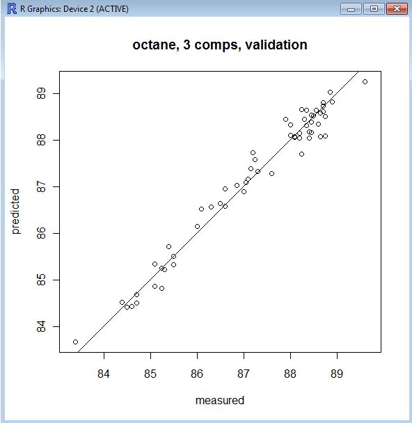
We will continue with more plots in the next post.
Tutorials of :
Bjorn-Helge Mevik
Norwegian University of Life Sciences
Ron Wehrens
Radboud University NijmegenTweet
To leave a comment for the author, please follow the link and comment on their blog: NIR-Quimiometría.
R-bloggers.com offers daily e-mail updates about R news and tutorials about learning R and many other topics. Click here if you're looking to post or find an R/data-science job.
Want to share your content on R-bloggers? click here if you have a blog, or here if you don't.