
Process and observation uncertainty explained with R
Want to share your content on R-bloggers? click here if you have a blog, or here if you don't.
Once up on a time I had grand ambitions of writing blog posts outlining all of the examples in the Ecological Detective.1 A few years ago I participated in a graduate seminar series where we went through many of the examples in this book. I am not a population biologist by trade but many of the concepts were useful for not only helping me better understand core concepts of statistical modelling, but also for developing an appreciation of the limits of your data. Part of this appreciation stems from understanding sources and causes of uncertainty in estimates. Perhaps in the future I will focus more blog topics on other examples from The Ecological Detective, but for now I’d like to discuss an example that has recently been of interest in my own research.
Over the past few months I have been working with some colleagues to evaluate statistical power of biological indicators. These analyses are meant to describe the certainty within which a given level of change in an indicator is expected over a period of time. For example, what is the likelihood of detecting a 50% decline over twenty years considering that our estimate of the indicators are influenced by uncertainty? We need reliable estimates of the uncertainty to answer these types of questions and it is often useful to categorize sources of variation. Hilborn and Mangel describe process and observation uncertainty as two primary categories of noise in a data measurements. Process uncertainty describes noise related to actual or real variation in a measurement that a model does not describe. For example, a model might describe response of an indicator to changing pollutant loads but we lack an idea of seasonal variation that occurs naturally over time. Observation uncertainty is often called sampling uncertainty and describes our ability to obtain a precise data measurement. This is a common source of uncertainty in ecological data where precision of repeated surveys may be affected by several factors, such as skill level of the field crew, precision of sampling devices, and location of survey points. The effects of process and observation uncertainty on data measurements are additive such that the magnitude of both can be separately estimated.
The example I’ll focus on is described on pages 59–61 (the theory) and 90–92 (an example with pseudocode) in The Ecological Detective. This example describes n approach for conceptualizing the effects of uncertainty on model estimates, as opposed to methods for quantifying certainty from actual data. For the most part, this blog is an exact replica of the example, although I have tried to include some additional explanation where I had difficulty understanding some of the concepts. Of course, I’ll also include R code since that’s the primary motivation for my blog.
We start with a basic population model that describes population change over time. This is a theoretical model that, in practice, should describe some actual population, but is very simple for the purpose of learning about sources of uncertainty. From this basic model, we simulate sources of uncertainty to get an idea of their exact influence on our data measurements. The basic model without imposing uncertainty is as follows:

where the population at time 


# simple pop model
proc_mod <- function(N_0 = 50, b = 20, s = 0.8, t = 50){

	N_out <- numeric(length = t)
	N_out[1] <- N_0

	for(step in 1:t)
		N_out[step + 1] <- s*N_out[step] + b

	out <- data.frame(steps = 1:t, Pop = N_out[-1])

	return(out)

}

est <- proc_mod()
The model is pretty straightforward. A for loop is used to estimate the population for time steps one to fifty with a starting population size of fifty at time zero. Each time step multiplies the population estimate from the previous time step and adds twenty new individuals. You may notice that the function could easily be vectorized, but I’ve used a for loop to account for sources of uncertainty that are dependent on previous values in the time series. This will be explained below but for now the model only describes the actual process.
The results are assigned to the est object and then plotted.
library(ggplot2)
ggplot(est, aes(steps, Pop)) +
	geom_point() +
	theme_bw() +
	ggtitle('N_0 = 50, s = 0.8, b = 20\n')
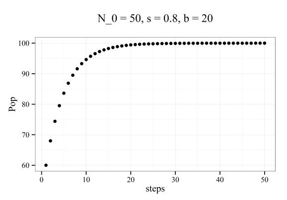
In a world with absolute certainty, an actual population would follow this trend if our model accurately described the birth and survivorship rates. Suppose our model provided an incomplete description of the population. Hilborn and Mangel (p. 59) suggest that birth rates, for example, may fluctuate from year to year. This fluctuation is not captured by our model and represents a source of process uncertainty, or uncertainty caused by an incomplete description of the process. We can assume that the effect of this process uncertainty is additive to the population estimate at each time step:

where the model remains the same but we’ve included an additional term, 

for loop is used because we can’t simulate uncertainty by adding a random vector all at once to the population estimates.
The original model is modified to include process uncertainty.
# simple pop model with process uncertainty
proc_mod2 <- function(N_0 = 50, b = 20, s = 0.8, t = 50,
        sig_w = 5){

	N_out <- numeric(length = t + 1)
	N_out[1] <- N_0

	sig_w <- rnorm(t, 0, sig_w)

	for(step in 1:t)
		N_out[step + 1] <- s*N_out[step] + b + sig_w[step]

	out <- data.frame(steps = 1:t, Pop = N_out[-1])

	return(out)

}

set.seed(2)
est2 <- proc_mod2()

# plot the estimates
ggt <- paste0('N_0 = 50, s = 0.8, b = 20, sig_w = ',formals(proc_mod)$sig_w,'\n')
ggplot(est2, aes(steps, Pop)) +
	geom_point() +
	theme_bw() +
	ggtitle(ggt)
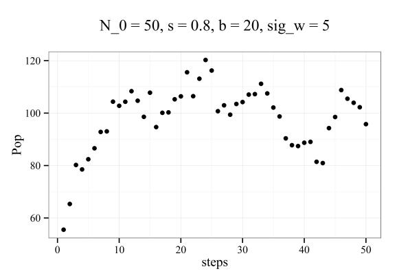
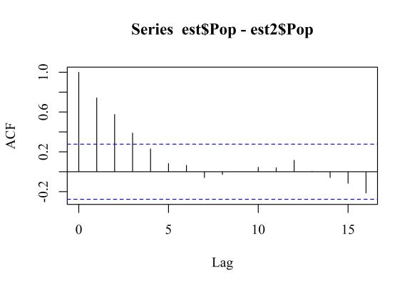
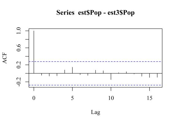
We see considerable variation from the original model now that we’ve included process uncertainty. Note that the process uncertainty in each estimate is dependent on the estimate prior, as described above. This creates uncertainty that, although random, follows a pattern throughout the time series. We can look at an auto-correlation plot of the new estimates minus the actual population values to get an idea of this pattern. Observations that are closer to one another in the time series are correlated, as expected.
Adding observation uncertainty is simpler in that the effect is not propagated throughout the time steps. Rather, the uncertainty is added after the time series is generated. This makes intuitive because the observation uncertainty describes sampling error. For example, if we have an instrument malfunction one year that creates an unreliable estimate we can fix the instrument to get a more accurate reading the next year. However, suppose we have a new field crew the following year that contributes to uncertainty (e.g., wrong species identification). This uncertainty is not related to the year prior. Computationally, the model is as follows:


where the model is identical to the deterministic model with the addition of observation uncertainty 
# model with observation uncertainty
proc_mod3 <- function(N_0 = 50, b = 20, s = 0.8, t = 50, sig_v = 5){

	N_out <- numeric(length = t)
	N_out[1] <- N_0

	sig_v <- rnorm(t, 0, sig_v)

	for(step in 1:t)
		N_out[step + 1] <- s*N_out[step] + b

	N_out <- N_out + c(NA,sig_v)

	out <- data.frame(steps = 1:t, Pop = N_out[-1])

	return(out)

}

# get estimates
set.seed(3)
est3 <- proc_mod3()

# plot
ggt <- paste0('N_0 = 50, s = 0.8, b = 20, sig_v = ',
        formals(proc_mod3)$sig_v,'\n')
ggplot(est3, aes(steps, Pop)) +
        geom_point() +
	theme_bw() +
	ggtitle(ggt)
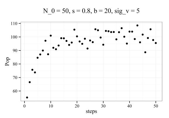
We can confirm that the observations are not correlated between the time steps, unlike the model with process uncertainty.
Now we can create a model that includes both process and observation uncertainty by combining the above functions. The function is slightly tweaked to return include a data frame with all estimates: process model only, process model with process uncertainty, process model with observation uncertainty, process model with process and observation uncertainty.
# combined function
proc_mod_all <- function(N_0 = 50, b = 20, s = 0.8, t = 50,
        sig_w = 5, sig_v = 5){

	N_out <- matrix(NA, ncol = 4, nrow = t + 1)
	N_out[1,] <- N_0

	sig_w <- rnorm(t, 0, sig_w)
	sig_v <- rnorm(t, 0, sig_v)

	for(step in 1:t){
		N_out[step + 1, 1] <- s*N_out[step] + b
		N_out[step + 1, 2] <- N_out[step, 1] + sig_w[step]
		}

	N_out[1:t + 1, 3]  <- N_out[1:t + 1, 1] + sig_v

	N_out[1:t + 1, 4]  <- N_out[1:t + 1, 2] + sig_v

	out <- data.frame(1:t,N_out[-1,])
	names(out) <- c('steps', 'mod_act', 'mod_proc', 'mod_obs', 'mod_all')

	return(out)

}

# create data
set.seed(2)
est_all <- proc_mod_all()

# plot the data
library(reshape2)
to_plo <- melt(est_all, id.var = 'steps')

# re-assign factor labels for plotting
to_plo$variable <- factor(to_plo$variable, levels = levels(to_plo$variable),
	labels = c('Actual','Pro','Obs','Pro + Obs'))

ggplot(to_plo, aes(steps, value)) +
	geom_point() +
	facet_wrap(~variable) +
	ylab('Pop. estimate') +
	theme_bw()
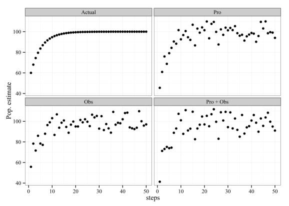
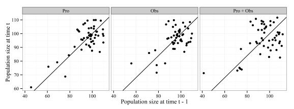
On the surface, the separate effects of process and observation uncertainty on the estimates is similar, whereas the effects of adding both maximizes the overall uncertainty. We can quantify the extent to which the sources of uncertainty influence the estimates by comparing observations at time 
# comparison of mods
# create vectors for pop estimates at time t (t_1) and t - 1 (t_0)
t_1 <- est_all[2:nrow(est_all),-1]
t_1 <- melt(t_1, value.name = 'val_1')
t_0 <- est_all[1:(nrow(est_all)-1),-1]
t_0 <- melt(t_0, value.name = 'val_0')

#combine for plotting
to_plo2 <- cbind(t_0,t_1[,!names(t_1) %in% 'variable',drop = F])
head(to_plo2)
##   variable   val_0    val_1
## 1  mod_act 60.0000 68.00000
## 2  mod_act 68.0000 74.40000
## 3  mod_act 74.4000 79.52000
## 4  mod_act 79.5200 83.61600
## 5  mod_act 83.6160 86.89280
## 6  mod_act 86.8928 89.51424

# re-assign factor labels for plotting
to_plo2$variable <- factor(to_plo2$variable, levels = levels(to_plo2$variable),
	labels = c('Actual','Pro','Obs','Pro + Obs'))

# we don't want to plot the first process model
sub_dat <- to_plo2$variable == 'Actual'
ggplot(to_plo2[!sub_dat,], aes(val_0, val_1)) +
	geom_point() +
	facet_wrap(~variable) +
	theme_bw() +
	scale_y_continuous('Population size at time t') +
	scale_x_continuous('Population size at time t - 1') +
	geom_abline(slope = 0.8, intercept = 20)
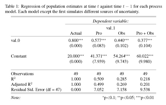
A tabular comparison of the regressions for each plot provides a quantitative measure of the effect of uncertainty on the model estimates.
library(stargazer)
mods <- lapply(
	split(to_plo2,to_plo2$variable),
	function(x) lm(val_1~val_0, data = x)
	)
stargazer(mods, omit.stat = 'f', title = 'Regression of population estimates at time $t$ against time $t - 1$ for each process model.  Each model except the first simulates different sources of uncertainty.', column.labels = c('Actual','Pro','Obs','Pro + Obs'), model.numbers = F)
The table tells us exactly what we would expect. Based on the r-squared values, adding more uncertainty decreases the explained variance of the models. Also note the changes in the parameter estimates. The actual model provides slope and intercept estimates identical to those we specified in the beginning (

It’s nice to use an arbitrary model where we can simulate effects of uncertainty, unlike situations with actual data where sources of uncertainty are not readily apparent. This example from The Ecological Detective is useful for appreciating the effects of uncertainty on parameter estimates in simple process models. I refer the reader to the actual text for more discussion regarding the implications of these analyses. Also, check out Ben Bolker’s text2 (chapter 11) for more discussion with R examples.
Cheers,
Marcus
1Hilborn R, Mangel M. 1997. The Ecological Detective: Confronting Models With Data. Monographs in Population Biology 28. Princeton University Press. Princeton, New Jersey. 315 pages.
2Bolker B. 2007. Ecological Models and Data in R. Princeton University Press. Princeton, New Jersey. 508 pages.

R-bloggers.com offers daily e-mail updates about R news and tutorials about learning R and many other topics. Click here if you're looking to post or find an R/data-science job.
Want to share your content on R-bloggers? click here if you have a blog, or here if you don't.