
On the carbon footprint of the NBA
Want to share your content on R-bloggers? click here if you have a blog, or here if you don't.
It’s no secret that I enjoy basketball, but I’ve often wondered about the carbon footprint that can be caused by 30 teams each playing an 82-game season. Ultimately, that’s 2460 air flights across the whole of the USA, each carrying 30+ individuals.
For these reasons, I decided to investigate the average distance travelled by each NBA team during the 2013-2014 NBA season. In order to do so, I had to obtain the game schedule for the whole 2013-2014 season, but also the distances between arenas in which games are played. While obtaining the regular season schedule was straightforward (a shameless copy and paste), for the distance between arenas, I first had to extract the coordinates of each arena, which could be achieved using the geocode function in the ggmap package.
Example: finding the coordinates of NBA arenas:
# find geocode location of a given NBA arena
library(maps)
library(mapdata)
library(ggmap)
geo.tag1 <- geocode('Bankers Life Fieldhouse')
geo.tag2 <- geocode('Madison Square Garden')
print(geo.tag1)
geo.tag1
        lon     lat
1 -86.15578 39.7639
Once the coordinate of all NBA arenas were obtained, we can use this information to compute the pairwise distance matrix between each NBA arena. However we first had to define a function to compute the distance between two pairs of latitude-longitude.
Computing the distance between two coordinate points:
# Function to calculate distance in kilometers between two points
# reference: http://andrew.hedges.name/experiments/haversine/
earth.dist <- function (lon1, lat1, lon2, lat2, R)
{
  rad <- pi/180
  a1 <- lat1 * rad
  a2 <- lon1 * rad
  b1 <- lat2 * rad
  b2 <- lon2 * rad
  dlon <- b2 - a2
  dlat <- b1 - a1
  a <- (sin(dlat/2))^2 + cos(a1) * cos(b1) * (sin(dlon/2))^2
  c <- 2 * atan2(sqrt(a), sqrt(1 - a))
  d <- R * c
  real.d <- min(abs((R*2) - d), d)
  return(real.d)
}
Using the function above and the coordinates of NBA arenas, the distance between any two given NBA arenas can be computed with the following lines of code.
Computing the distance matrix between all NBA arenas:
# compute distance between each NBA arena
dist <- c()
R <- 6378.145 # define radius of earth in km
lon1 <- geo.tag1$lon
lat1 <- geo.tag1$lat
lon2 <- geo.tag2$lon
lat2 <- geo.tag2$lat
dist <- earth.dist(lon1, lat1, lon2, lat2, R)

print(dist)
485.6051
By performing this operation on all pairs of NBA teams, we can compute a distance matrix, which can be used in conjunction with the 2013-2014 regular season schedule to compute the total distance travelled by each NBA teams. Finally, all that was left was to visualize the data in an attractive manner. I find the googleVis is a great resource for that, as it provides a convenient interface between R and the Google Chart Tools API. Because wordpress.com does not support javascript, you can view the interactive graph by clicking on the image below.
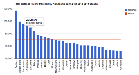
Total distance (in km) travelled by all NBA teams during the 2013-2014 NBA regular season
Incredibly, we see that the aggregate number of kilometers travelled by NBA teams amounts to 2,108,806 kms! I hope the players have some kind of frequent flyer card…We can take this a step further by computing the amount of CO2 emitted by each NBA team during the 2013-2014 season. The NBA charters standard A319 Airbus planes, which according to the Airbus website emits an average of 9.92 kg of CO2 per km. Again, you can view the interactive graph of CO2 by clicking on the image below.
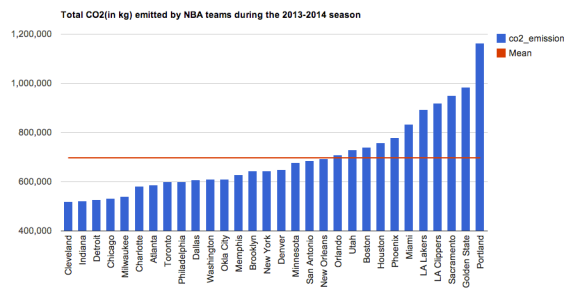
Total amount of CO2 (in kg) consummed by all NBA teams during the 2013-2014 NBA regular season
Not surprisingly, Oregon and California-based teams travel and pollute the most, since the NBA is mid-east / east coast heavy in its distribution of teams. It is somewhat ironic that the hipster / recycle-crazy / eco-friendly citizens of Portland are also the host of the most polluting NBA team 🙂
What is also interesting is to plot the trail of flights (or pollution) achieved by the NBA throught the season.

Great circle maps of all airplane flights completed by NBA teams during the 2013-2014 regular season.
I’ve been thinking about designing an algorithm that finds the NBA season schedule with minimal carbon footprint, which is essentially an optimization problem. The only issue is that there are a huge amount of restrictions to consider, such as christmas day games, first day of season games etc… More on that later.
As usual, all the relevant code for this analysis can be found on my github account.

R-bloggers.com offers daily e-mail updates about R news and tutorials about learning R and many other topics. Click here if you're looking to post or find an R/data-science job.
Want to share your content on R-bloggers? click here if you have a blog, or here if you don't.