
Fitting Polynomial Regression in R
Want to share your content on R-bloggers? click here if you have a blog, or here if you don't.
A linear relationship between two variables x and y is one of the most common, effective and easy assumptions to make when trying to figure out their relationship. Sometimes however, the true underlying relationship is more complex than that, and this is when polynomial regression comes in to help.
Let see an example from economics: Suppose you would like to buy a certain quantity q of a certain product. If the unit price is p, then you would pay a total amount y. This is a typical example of a linear relationship. Total price and quantity are directly proportional. To plot it we would write something like this:
p <- 0.5
q <- seq(0,100,1)
y <- p*q
plot(q,y,type='l',col='red',main='Linear relationship')
The plot will look like this:

Now, this is a good approximation of the true relationship between y and q, however when buying and selling we might want to consider some other relevant information, like: Buying significant quantities it is likely that we can ask and get a discount, or buying more and more of a certain good we might be pushing the price up.
This can lead to a scenario like this one where the total cost is no longer a linear function of the quantity:
y <- 450 + p*(q-10)^3
plot(q,y,type='l',col='navy',main='Nonlinear relationship',lwd=3)
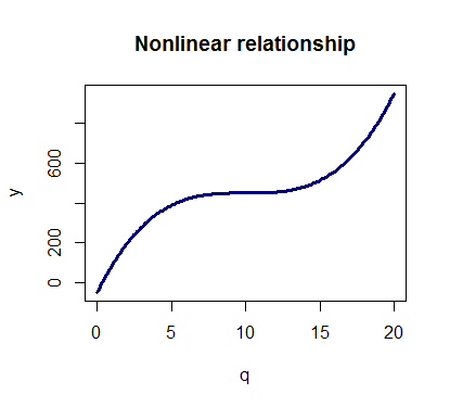
With polynomial regression we can fit models of order n > 1 to the data and try to model nonlinear relationships.
How to fit a polynomial regression
First, always remember use to set.seed(n) when generating pseudo random numbers. By doing this, the random number generator generates always the same numbers.
set.seed(20)
Predictor (q). Use seq for generating equally spaced sequences fast
q <- seq(from=0, to=20, by=0.1)
Value to predict (y):
y <- 500 + 0.4 * (q-10)^3
Some noise is generated and added to the real signal (y):
noise <- rnorm(length(q), mean=10, sd=80)
noisy.y <- y + noise
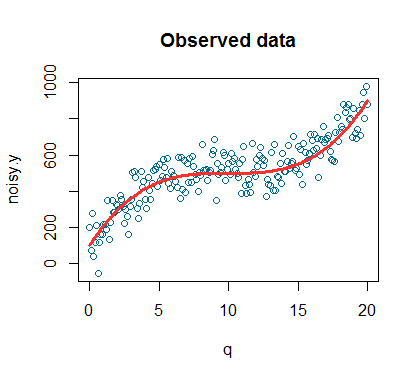
Plot of the noisy signal:
plot(q,noisy.y,col='deepskyblue4',xlab='q',main='Observed data')
lines(q,y,col='firebrick1',lwd=3)
This is the plot of our simulated observed data. The simulated datapoints are the blue dots while the red line is the signal (signal is a technical term that is often used to indicate the general trend we are interested in detecting).
Our model should be something like this: y = a*q + b*q2 + c*q3 + cost
Let’s fit it using R. When fitting polynomials you can either use
model <- lm(noisy.y ~ poly(q,3))
Or
model <- lm(noisy.y ~ x + I(X^2) + I(X^3))
However, note that q, I(q^2) and I(q^3) will be correlated and correlated variables can cause problems. The use of poly() lets you avoid this by producing orthogonal polynomials, therefore I’m going to use the first option.
summary(model)

Call:
lm(formula = noisy.y ~ poly(q, 3))

Residuals:
     Min       1Q   Median       3Q      Max
-212.326  -51.186    4.276   61.485  165.960

Coefficients:
            Estimate Std. Error t value Pr(>|t|)
(Intercept)  513.615      5.602   91.69   <2e-16 ***
poly(q, 3)1 2075.899     79.422   26.14   <2e-16 ***
poly(q, 3)2 -108.004     79.422   -1.36    0.175
poly(q, 3)3  864.025     79.422   10.88   <2e-16 ***
---
Signif. codes:  0 ‘***’ 0.001 ‘**’ 0.01 ‘*’ 0.05 ‘.’ 0.1 ‘ ’ 1

Residual standard error: 79.42 on 197 degrees of freedom
Multiple R-squared:  0.8031,	Adjusted R-squared:  0.8001
F-statistic: 267.8 on 3 and 197 DF,  p-value:  0
By using the confint() function we can obtain the confidence intervals of the parameters of our model.
Confidence intervals for model parameters:
confint(model, level=0.95)

                2.5 %     97.5 %
(Intercept)  502.5676  524.66261
poly(q, 3)1 1919.2739 2232.52494
poly(q, 3)2 -264.6292   48.62188
poly(q, 3)3  707.3999 1020.65097
Plot of fitted vs residuals. No clear pattern should show in the residual plot if the model is a good fit
plot(fitted(model),residuals(model))

Overall the model seems a good fit as the R squared of 0.8 indicates. The coefficients of the first and third order terms are statistically significant as we expected. Now we can use the predict() function to get the fitted values and the confidence intervals in order to plot everything against our data.
Predicted values and confidence intervals:
predicted.intervals <- predict(model,data.frame(x=q),interval='confidence',
                               level=0.99)
Add lines to the existing plot:
lines(q,predicted.intervals[,1],col='green',lwd=3)
lines(q,predicted.intervals[,2],col='black',lwd=1)
lines(q,predicted.intervals[,3],col='black',lwd=1)
Add a legend:
legend("bottomright",c("Observ.","Signal","Predicted"),
       col=c("deepskyblue4","red","green"), lwd=3)
Here is the plot:

We can see that our model did a decent job at fitting the data and therefore we can be satisfied with it.
A word of caution: Polynomials are powerful tools but might backfire: in this case we knew that the original signal was generated using a third degree polynomial, however when analyzing real data, we usually know little about it and therefore we need to be cautious because the use of high order polynomials (n > 4) may lead to over-fitting. Over-fitting happens when your model is picking up the noise instead of the signal: even though your model is getting better and better at fitting the existing data, this can be bad when you are trying to predict new data and lead to misleading results.
A gist with the full code for this example can be found here.
Thank you for reading this post, leave a comment below if you have any question.
R-bloggers.com offers daily e-mail updates about R news and tutorials about learning R and many other topics. Click here if you're looking to post or find an R/data-science job.
Want to share your content on R-bloggers? click here if you have a blog, or here if you don't.