Data Profiling in R

In 2006 UserR conference Jim Porzak gave a presentation on data profiling with R. He showed how to draw summary panels of the data using a combination of grid and base graphics.

Unfortunately the code has not (yet) been released as a package, so when I recently needed to quickly review several datasets at the beginning of an analysis project I started to look for alternatives. A quick search revealed two options that offer similar functionality: r2lUniv package and describe() function in Hmisc package.

r2lUniv

r2lUniv package performs quick analysis either on a single variable or on a dataframe by computing several statistics (frequency, centrality, dispersion, graph) for each variable and outputs the results in a LaTeX format. The output varies depending on the variable type.

> library(r2lUniv)

One can specify the text to be inserted in front of each section.

> textBefore <- paste("\\subsection{", names(mtcars),
+     "}", sep = "")
> rtlu(mtcars, "fileOut.tex", textBefore = textBefore)

The function rtluMainFile generates a LaTeX main document design and allows to further customise the report.

> text <- "\\input{fileOut.tex}"
> rtluMainFile("r2lUniv_report.tex", text = text)

The resulting tex-file can then be converted into pdf.

> library(tools)
> texi2dvi("r2lUniv_report.tex", pdf = TRUE, clean = TRUE)

A sample output for the mpg-variable:

The final pdf-output can be seen here: r2lUniv_report.pdf.

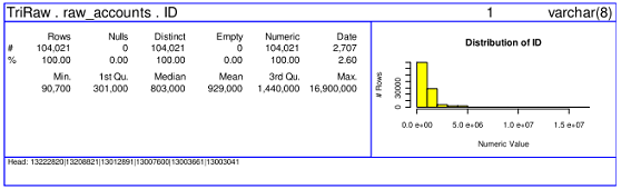
Hmisc

The describe function in Hmisc package determines whether the variable is character, factor, category, binary, discrete numeric, and continuous numeric, and prints a concise statistical summary according to each. The latex report also includes a spike histogram displaying the frequency counts.

> library(Hmisc)

> db <- describe(mtcars, size = "normalsize")

The easiest and fastest way is to print the results to the console.

> db$mpg
mpg
      n missing  unique    Mean     .05     .10     .25     .50
     32       0      25   20.09   12.00   14.34   15.43   19.20
    .75     .90     .95
  22.80   30.09   31.30

lowest : 10.4 13.3 14.3 14.7 15.0
highest: 26.0 27.3 30.4 32.4 33.9

Alternatively, one can convert the describe object into a LaTeX file.

> x <- latex(db, file = "describe.tex")

cat is used to generate the tex-report.

> text2 <- "\\documentclass{article}\n\\usepackage{relsize,setspace}\n\\begin{document}\n\\input{describe.tex} \n\\end{document}"
> cat(text2, file = "Hmisc_describe_report.tex")

> library(tools)
> texi2dvi("Hmisc_describe_report.tex", pdf = TRUE)

A sample output for the mpg-variable:

The final pdf-report can be seen here: Hmisc_describe_report.pdf.

Conclusion

Both of the functions provide similar snapshots of the data, however I prefer the describe function for its more concise output, and also for the option to print the analysis to the console. Whilst I like the summary plots generated by r2lUniv I find them hard to read in the pdf-report because of the small font-size of the labels.