
Data Mining in A Nutshell
[This article was first published on Econometric Sense, and kindly contributed to R-bloggers]. (You can report issue about the content on this page here)
Want to share your content on R-bloggers? click here if you have a blog, or here if you don't.
Want to share your content on R-bloggers? click here if you have a blog, or here if you don't.
# The following code may look rough, but simply paste into R or
# a text editor (especially Notepad++) and it will look
# much better.
# PROGRAM NAME: MACHINE_LEARNING_R
# DATE: 4/19/2010
# AUTHOR : MATT BOGARD
# PURPOSE: BASIC EXAMPLES OF MACHINE LEARNING IMPLEMENTATIONS IN R
# DATA USED: GENERATED VIA SIMULATION IN PROGRAM
# COMMENTS: CODE ADAPTED FROM : Joshua Reich ([email protected]) April 2, 2009
# SUPPORT VECTOR MACHINE CODE ALSO BASED ON :
# ëSupport Vector Machines in Rî Journal of Statistical Software April 2006 Vol 15 Issue 9
#
# CONTENTS: SUPPORT VECTOR MACHINES
# DECISION TREES
# NEURAL NETWORK
# load packages
library(rpart)
library(MASS)
library(class)
library(e1071)
# get data
# A simple function for producing n random samples
# from a multivariate normal distribution with mean mu
# and covariance matrix sigma
rmulnorm <- function (n, mu, sigma) {
M <- t(chol(sigma))
d <- nrow(sigma)
Z <- matrix(rnorm(d*n),d,n)
t(M %*% Z + mu)
}
# Produce a confusion matrix
# there is a potential bug in here if columns are tied for ordering
cm <- function (actual, predicted)
{
t<-table(predicted,actual)
t[apply(t,2,function(c) order(-c)[1]),]
}
# Total number of observations
N <- 1000 * 3# Number of training observations
Ntrain <- N * 0.7 # The data that we will be using for the demonstration consists
# of a mixture of 3 multivariate normal distributions. The goal
# is to come up with a classification system that can tell us,
# given a pair of coordinates, from which distribution the data
# arises.
A <- rmulnorm (N/3, c(1,1), matrix(c(4,-6,-6,18), 2,2))
B <- rmulnorm (N/3, c(8,1), matrix(c(1,0,0,1), 2,2))
C <- rmulnorm (N/3, c(3,8), matrix(c(4,0.5,0.5,2), 2,2))
data <- data.frame(rbind (A,B,C))
colnames(data) <- c('x', 'y')
data$class <- c(rep('A', N/3), rep('B', N/3), rep('C', N/3))
# Lets have a look
plot_it <- function () {plot (data[,1:2], type=’n’)
points(A, pch=’A’, col=’red’)
points(B, pch=’B’, col=’blue’)
points(C, pch=’C’, col=’orange’)
}
plot_it()

# Randomly arrange the data and divide it into a training
# and test set.
data <- data[sample(1:N),]train <- data[1:Ntrain,]
test <- data[(Ntrain+1):N,]
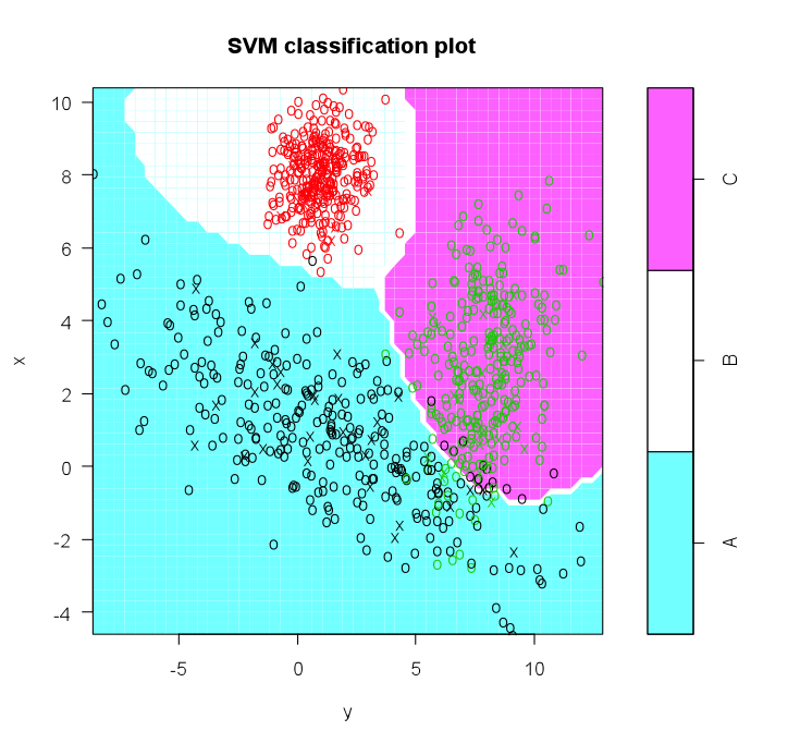
# SVM
# Support vector machines take the next step from LDA/QDA. However
# instead of making linear voronoi boundaries between the cluster
# means, we concern ourselves primarily with the points on the
# boundaries between the clusters. These boundary points define
# the ‘support vector’. Between two completely separable clusters
# there are two support vectors and a margin of empty space
# between them. The SVM optimization technique seeks to maximize
# the margin by choosing a hyperplane between the support vectors
# of the opposing clusters. For non-separable clusters, a slack
# constraint is added to allow for a small number of points to
# lie inside the margin space. The Cost parameter defines how
# to choose the optimal classifier given the presence of points
# inside the margin. Using the kernel trick (see Mercer’s theorem)
# we can get around the requirement for linear separation
# by representing the mapping from the linear feature space to
# some other non-linear space that maximizes separation. Normally
# a kernel would be used to define this mapping, but with the
# kernel trick, we can represent this kernel as a dot product.
# In the end, we don’t even have to define the transform between
# spaces, only the dot product distance metric. This leaves
# this algorithm much the same, but with the addition of
# parameters that define this metric. The default kernel used
# is a radial kernel, similar to the kernel defined in my
# kernel method example. The addition is a term, gamma, to
# add a regularization term to weight the importance of distance.
s <- svm( I(factor(class)) ~ x + y, data = train, cost = 100, gama = 1)
s # print model results
#plot model and classification-my code not originally part of this
plot(s,test)
(m <- cm(train$class, predict(s)))
1 – sum(diag(m)) / sum(m)
(m <- cm(test$class, predict(s, test[,1:2])))
1 – sum(diag(m)) / sum(m)
# Recursive Partitioning / Regression Trees
# rpart() implements an algorithm that attempts to recursively split
# the data such that each split best partitions the space according
# to the classification. In a simple one-dimensional case with binary
# classification, the first split will occur at the point on the line
# where there is the biggest difference between the proportion of
# cases on either side of that point. The algorithm continues to
# split the space until a stopping condition is reached. Once the
# tree of splits is produced it can be pruned using regularization
# parameters that seek to ameliorate overfitting.
names(train)names(test)
(r <- rpart(class ~ x + y, data = train)) plot(r) text(r) summary(r) plotcp(r) printcp(r) rsq.rpart(r)

cat(“\nTEST DATA Error Matrix – Counts\n\n”)
print(table(predict(r, test, type=”class”),test$class, dnn=c(“Predicted”, “Actual”)))
# Here we look at the confusion matrix and overall error rate from applying
# the tree rules to the training data.
predicted <- as.numeric(apply(predict(r), 1, function(r) order(-r)[1]))
(m <- cm (train$class, predicted))
1 – sum(diag(m)) / sum(m)
# Neural Network
# Recall from the heuristic on data mining and machine learning , a neural network is # a nonlinear model of complex relationships composed of multiple ‘hidden’ layers
# (similar to composite functions)
# Build the NNet model.
require(nnet, quietly=TRUE)
crs_nnet <- nnet(as.factor(class) ~ ., data=train, size=10, skip=TRUE, trace=FALSE, maxit=1000)
# Print the results of the modelling.
print(crs_nnet)
print(“
Network Weights:
“)
print(summary(crs_nnet))
# Evaluate Model Performance
# Generate an Error Matrix for the Neural Net model.
# Obtain the response from the Neural Net model.
crs_pr <- predict(crs_nnet, train, type="class")
# Now generate the error matrix.
table(crs_pr, train$class, dnn=c(“Predicted”, “Actual”))
# Generate error matrix showing percentages.
round(100*table(crs_pr, train$class, dnn=c(“Predicted”, “Actual”))/length(crs_pr))
Calucate overall error percentage.
print( “Overall Error Rate”)
(function(x){ if (nrow(x) == 2) cat((x[1,2]+x[2,1])/sum(x)) else cat(1-(x[1,rownames(x)])/sum(x))}) (table(crs_pr, train$class, dnn=c(“Predicted”, “Actual”)))
To leave a comment for the author, please follow the link and comment on their blog: Econometric Sense.
R-bloggers.com offers daily e-mail updates about R news and tutorials about learning R and many other topics. Click here if you're looking to post or find an R/data-science job.
Want to share your content on R-bloggers? click here if you have a blog, or here if you don't.