Bootstrap, strap-on, anal-yzing… statistics is getting weirder by the moment
Want to share your content on R-bloggers? click here if you have a blog, or here if you don't.
I have spent the better portion of the day trying to get a bootstrap working. I have adapter a pre-written bootstrap function, but I wanted to use a generic function, mostly for reaping fame and glory. My hypothesis was that writing a hand-written, unoptimized function will consume more computer time than the generic, presumably optimized, boot() function. Was I wrong!
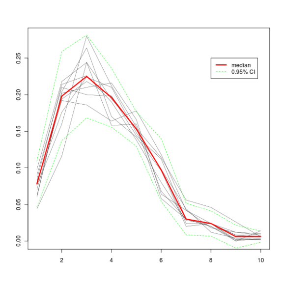
In this example, I random sample (with replacement) a vector of n values and store them in a matrix. These values that are written to the matrix are percent of values of our initial vector values that are smaller or equal to the bin number (see the code). Once we’ve got all the values, we can calculate the median by columns for further tinkering. There’s a lot of material covering bootstrapping on the Internet, but for a quick reference, see this Wikipedia entry. At this StackOverflow thread, Aniko provided me with valuable information on what I was doing wrong.
This is the code I used – first part is the hand written function, and the second part is my attempt at cracking the matter with a generic function.
require(Hmisc)

#generate fake data
data <- rchisq(500, df = 12)

#create bins
binx <- cut(data, breaks = 10)
binx <- levels(binx)
binx <- sub("^.*\\,", "", binx)
binx <- as.numeric(substr(binx, 1, nchar(binx) - 1))

#pre-allocate a matrix to be filled with samples
num.boots <- 10
output <- matrix(NA, nrow = num.boots, ncol = length(binx))

#do random sampling from the vector and calculate percent
#of values equal or smaller to the bin number (i)

for (i in 1:num.boots) {
 data.sample <- sample(data, size = length(data), replace = TRUE)
 data.cut <- cut(x = data.sample, breaks = 10)
 data.cut <- table(data.cut)/sum(table(data.cut))
 output[i, ] <- data.cut
}

#do some plotting
plot(1:10, seq(0, max(output), length.out = nrow(output)), type = "n", xlab = "", ylab = "")

for (i in 1:nrow(output)) {
 lines(1:10, output[i, 1:nrow(output)], lwd = "0.5")
}
output.median <- apply(output, 2, median)
output.sd <- apply(output, 2, sd)
sd.up <- output.median + output.sd * 1.96
sd.down <- output.median - output.sd * 1.96

lines(output.median, col="red", lwd = 3)
lines(sd.up, lty="dashed", col="green")
lines(sd.down, lty="dashed", col="green")
legend(x = 8, y = 0.25, legend = c("median", "0.95% CI"), col = c("red", "green"), lty = c("solid", "dashed"), lwd = c(3, 1))
All this produces this graph.
We can then try the power of the generic boot::boot() function that comes with the R core packages. The fun part of doing a bootstraping with the boot() function is to figure out how to write the statistic function correctly. If you look at the boot() help page (?boot) you will notice that you need to provide at least two parameters to the statistic argument: data and an index parameter. Help page says that the index parameter is a vector, which is a bit confusing from where I sit. In other words, this is actually a “an empty object” (let’s call the object i for now) that tells the boot() how to crawl over your data. If your data is in a form of a vector, you will place the index as you would use to subset a vector – object[i]. If it’s a data.frame and you want to re-sample rows, you would call object[i, ]… Let’s see a working example, things may be clearer there.
pairboot <- function(data, i, binx) {
 data.cut <- cut(x = data[i], breaks = 10)
 data.cut <- table(data.cut)/sum(table(data.cut))
 return(data.cut)
}
Notice the data[i] in the function. This will tell the boot() function to extract i elements of the data. If we had a data.frame, and rows were what we wanted to sample randomly, we would have written data[i, ].
And now we call the boot function to perform 10 “boots” on our data.
library(boot)
booty.call <- boot(data = data, statistic = pairboot, R = 10, binx = binx)
And here is the code to plot the output of the boot object (actually, it’s the print.boot object!). If you don’t believe me, try it on your own and see if you get a similar picture as above.
plot(1:10, seq(0, 1.5 * max(booty.call$t0), length.out = nrow(booty.call$t)), type = "n", xlab = "", ylab = "")
apply(booty.call$t, 1, function(x) lines(x, lwd = 0.5))
booty.call.median <- apply(booty.call$t, 2, median)
booty.call.sd <- apply(booty.call$t, 2, sd)
booty.call.sd.up <- booty.call.median + booty.call.sd * 1.96
booty.call.sd.down <- booty.call.median - booty.call.sd * 1.96
lines(booty.call.median, col="red", lwd = 3)
lines(booty.call.sd.up, lty="dashed", col="green")
lines(booty.call.sd.down, lty="dashed", col="green")
legend(x = 8, y = 0.25, legend = c("median", "0.95% CI"), col = c("red", "green"), lty = c("solid", "dashed"), lwd = c(3, 1))
The plot thickens!
Have I, by doing a bootstrap with a generic function, profited time-wise at all? Here are the elapse times for 10000 iterations for our hand written bootstrap function and the generic, respectively.
# user  system elapsed
#20.045   0.664  22.821


# user  system elapsed
#20.382   0.612  22.097
So you can see, I profit by 0.724 seconds. Was it worth it? ![]() I can, for the moment, only wonder if I could improve the generic function to beat the hand-written one. Does anyone skilled in optimizing chip in any tips?
I can, for the moment, only wonder if I could improve the generic function to beat the hand-written one. Does anyone skilled in optimizing chip in any tips?
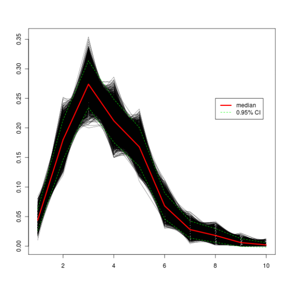
And here’s how a graph with 10000 iterations looks like. The green dashed lines represent a 95% confidence interval, which means that 95% of iterations fall between those two lines.
R-bloggers.com offers daily e-mail updates about R news and tutorials about learning R and many other topics. Click here if you're looking to post or find an R/data-science job.
Want to share your content on R-bloggers? click here if you have a blog, or here if you don't.


