
Bangalore workshop [ಬೆಂಗಳೂರು ಕಾರ್ಯಾಗಾರ]
Want to share your content on R-bloggers? click here if you have a blog, or here if you don't.
 Second day at the Indo-French Centre for Applied Mathematics and the workshop. Maybe not the most exciting day in terms of talks (as I missed the first two plenary sessions by (a) oversleeping and (b) running across the campus!). However I had a neat talk with another conference participant that led to [what I think are] interesting questions… (And a very good meal in a local restaurant as the guest house had not booked me for dinner!)
To wit: given a target like
 \prod_{i=1}^n \dfrac{1-\exp(-\lambda y_i)}{\lambda}\quad (*)")
the simulation of λ can be demarginalised into the simulation of
\propto \lambda \exp(-\lambda) \prod_{i=1}^n \exp(-\lambda z_i) \mathbb{I}(z_i\le y_i)")
where z is a latent (and artificial) variable. This means a Gibbs sampler simulating λ given z and z given λ can produce an outcome from the target (*). Interestingly, another completion is to consider that the zi‘s are U(0,yi) and to see the quantity
 \propto \lambda \exp(-\lambda) \prod_{i=1}^n \exp(-\lambda z_i) \mathbb{I}(z_i\le y_i)")
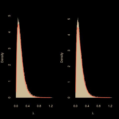
as an unbiased estimator of the target. What’s quite intriguing is that the quantity remains the same but with different motivations: (a) demarginalisation versus unbiasedness and (b) zi Exp(λ) versus zi U(0,yi). The stationary is the same, as shown by the graph below, the core distributions are [formally] the same, … but the reasoning deeply differs.
Obviously, since unbiased estimators of the likelihood can be justified by auxiliary variable arguments, this is not in fine a big surprise. Still, I had not though of the analogy between demarginalisation and unbiased likelihood estimation previously.Here are the R procedures if you are interested:
n=29
y=rexp(n)

T=10^5

#MCMC.1
lam=rep(1,T)

z=runif(n)*y
for (t in 1:T){

  lam[t]=rgamma(1,shap=2,rate=1+sum(z))
  z=-log(1-runif(n)*(1-exp(-lam[t]*y)))/lam[t]
  }

#MCMC.2
fam=rep(1,T)

z=runif(n)*y
for (t in 1:T){

  fam[t]=rgamma(1,shap=2,rate=1+sum(z))
  z=runif(n)*y
  }
Filed under: pictures, R, Running, Statistics, Travel, University life, Wines Tagged: auxiliary variable, Bangalore, demarginalisation, Gibbs sampler, IFCAM, Indian Institute of Science, unbiased estimation

R-bloggers.com offers daily e-mail updates about R news and tutorials about learning R and many other topics. Click here if you're looking to post or find an R/data-science job.
Want to share your content on R-bloggers? click here if you have a blog, or here if you don't.