
Zero Counts in dplyr
Want to share your content on R-bloggers? click here if you have a blog, or here if you don't.
Here’s a feature of dplyr that occasionally bites me (most recently while making these graphs). It’s about to change mostly for the better, but is also likely to bite me again in the future. If you want to follow along there’s a GitHub repo with the necessary code and data.
Say we have a data frame or tibble and we want to get a frequency table or set of counts out of it. In this case, each row of our data is a person serving a congressional term for the very first time, for the years 2013 to 2019. We have information on the term year, the party of the representative, and whether they are a man or a woman.
library(tidyverse)

## Hex colors for sex
sex_colors <- c("#E69F00", "#993300")

## Hex color codes for Dem Blue and Rep Red
party_colors <- c("#2E74C0", "#CB454A")

## Group labels
mf_labs <- tibble(M = "Men", F = "Women")

theme_set(theme_minimal())

## Character vectors only, by default
df <- read_csv("data/fc_sample.csv")

df

#> > df
#> # A tibble: 280 x 4
#>      pid start_year party      sex
#>    <int> <date>     <chr>      <chr>
#>  1  3160 2013-01-03 Republican M
#>  2  3161 2013-01-03 Democrat   F
#>  3  3162 2013-01-03 Democrat   M
#>  4  3163 2013-01-03 Republican M
#>  5  3164 2013-01-03 Democrat   M
#>  6  3165 2013-01-03 Republican M
#>  7  3166 2013-01-03 Republican M
#>  8  3167 2013-01-03 Democrat   F
#>  9  3168 2013-01-03 Republican M
#> 10  3169 2013-01-03 Democrat   M
#> # ... with 270 more rows
When we load our data into R with read_csv, the columns for party and sex are parsed as character vectors. If you’ve been around R for any length of time, and especially if you’ve worked in the tidyverse framework, you’ll be familiar with the drumbeat of “stringsAsFactors=FALSE”, by which we avoid classing character variables as factors unless we have a good reason to do so (there are several good reasons), and we don’t do so by default. Thus our df tibble shows us <chr> instead of <fct> for party and sex.
Now, let’s say we want a count of the number of men and women elected by party in each year. (Congressional elections happen every two years.) We write a little pipeline to group the data by year, party, and sex, count up the numbers, and calculate a frequency that’s the proportion of men and women elected that year within each party. That is, the frequencies of M and F will sum to 1 for each party in each year.
df %>%
    group_by(start_year, party, sex) %>%
    summarize(N = n()) %>%
    mutate(freq = N / sum(N))

#> # A tibble: 14 x 5
#> # Groups:   start_year, party [8]
#>    start_year party      sex       N   freq
#>    <date>     <chr>      <chr> <int>  <dbl>
#>  1 2013-01-03 Democrat   F        21 0.362
#>  2 2013-01-03 Democrat   M        37 0.638
#>  3 2013-01-03 Republican F         8 0.101
#>  4 2013-01-03 Republican M        71 0.899
#>  5 2015-01-03 Democrat   M         1 1
#>  6 2015-01-03 Republican M         5 1
#>  7 2017-01-03 Democrat   F         6 0.24
#>  8 2017-01-03 Democrat   M        19 0.76
#>  9 2017-01-03 Republican F         2 0.0667
#> 10 2017-01-03 Republican M        28 0.933
#> 11 2019-01-03 Democrat   F        33 0.647
#> 12 2019-01-03 Democrat   M        18 0.353
#> 13 2019-01-03 Republican F         1 0.0323
#> 14 2019-01-03 Republican M        30 0.968
You can see that, in 2015, neither party had a woman elected to Congress for the first time. Thus, the freq is 1 in row 5 and row 6. But you can also see that, because there are no observed Fs in 2015, they don’t show up in the table at all. The zero values are dropped. These rows, call them 5' and 6' don’t appear:
#>     start_year party      sex       N freq
#>  5' 2015-01-03 Democrat   F         0 0
#>  6' 2015-01-03 Republican F         0 0
How is that going to bite us? Let’s add some graphing instructions to the pipeline, first making a stacked column chart:
df %>%
    group_by(start_year, party, sex) %>%
    summarize(N = n()) %>%
    mutate(freq = N / sum(N)) %>%
    ggplot(aes(x = start_year,
               y = freq,
               fill = sex)) +
    geom_col() +
    scale_y_continuous(labels = scales::percent) +
    scale_fill_manual(values = sex_colors, labels = c("Women", "Men")) +
    labs(x = "Year", y = "Percent", fill = "Group") +
    facet_wrap(~ party)

ggsave("figures/df_chr_col.png")

Stacked column chart based on character-encoded values.
That looks fine. You can see in each panel the 2015 column is 100% Men. If we were working on this a bit longer we’d polish up the x-axis so that the dates were centered under the columns. But as an exploratory plot it’s fine.
But let’s say that, instead of a column plot, you looked at a line plot instead. This would be a natural thing to do given that time is on the x-axis and so you’re looking at a trend, albeit one over a small number of years.
df %>%
    group_by(start_year, party, sex) %>%
    summarize(N = n()) %>%
    mutate(freq = N / sum(N)) %>%
    ggplot(aes(x = start_year,
               y = freq,
               color = sex)) +
    geom_line(size = 1.1) +
    scale_y_continuous(labels = scales::percent) +
    scale_color_manual(values = sex_colors, labels = c("Women", "Men")) +
    guides(color = guide_legend(reverse = TRUE)) +
    labs(x = "Year", y = "Percent", color = "Group") +
    facet_wrap(~ party)

ggsave("figures/df_chr_line.png")

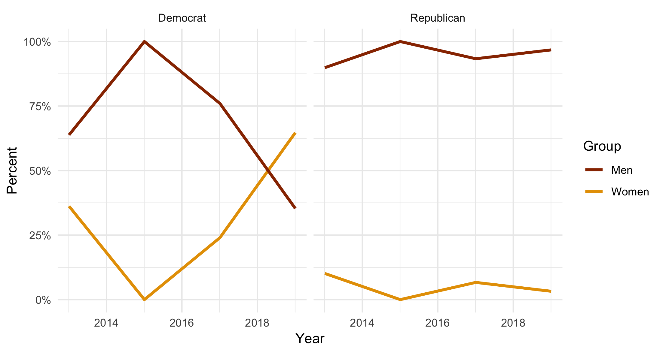
A line graph based on character-encoded variables for party and sex. The trend line for Women joins up the observed (or rather, the included) values, which don’t include the zero values for 2015.
That’s not right. The line segments join up the data points in the summary tibble, but because those don’t include the zero-count rows in the case of women, the lines join the 2013 and 2017 values directly. So we miss that the count (and thus the frequency) went to zero in that year.
This issue has been recognized in dplyr for some time. It happened whether your data was encoded as character or as a factor. There’s a huge thread about it in the development version on GitHub, going back to 2014. In the upcoming version 0.8 release of dplyr, the behavior for zero-count rows will change, but as far as I can make out it will change for factors only. Let’s see what happens when we change the encoding of our data frame. We’ll make a new one, called df_f.
df_f <- df %>% modify_if(is.character, as.factor)

df_f %>%
    group_by(start_year, party, sex) %>%
    tally()

#> # A tibble: 16 x 4
#> # Groups:   start_year, party [8]
#>    start_year party      sex       n
#>    <date>     <fct>      <fct> <int>
#>  1 2013-01-03 Democrat   F        21
#>  2 2013-01-03 Democrat   M        37
#>  3 2013-01-03 Republican F         8
#>  4 2013-01-03 Republican M        71
#>  5 2015-01-03 Democrat   F         0
#>  6 2015-01-03 Democrat   M         1
#>  7 2015-01-03 Republican F         0
#>  8 2015-01-03 Republican M         5
#>  9 2017-01-03 Democrat   F         6
#> 10 2017-01-03 Democrat   M        19
#> 11 2017-01-03 Republican F         2
#> 12 2017-01-03 Republican M        28
#> 13 2019-01-03 Democrat   F        33
#> 14 2019-01-03 Democrat   M        18
#> 15 2019-01-03 Republican F         1
#> 16 2019-01-03 Republican M        30
Now we have party and sex encoded as unordered factors. This time, our zero rows are present (here as rows 5 and 7). The grouping and summarizing operation has preserved all the factor values by default, instead of dropping the ones with no observed values in any particular year. Let’s run our line graph code again:
df_f %>%
    group_by(start_year, party, sex) %>%
    summarize(N = n()) %>%
    mutate(freq = N / sum(N)) %>%
    ggplot(aes(x = start_year,
               y = freq,
               color = sex)) +
    geom_line(size = 1.1) +
    scale_y_continuous(labels = scales::percent) +
    scale_color_manual(values = sex_colors, labels = c("Women", "Men")) +
    guides(color = guide_legend(reverse = TRUE)) +
    labs(x = "Year", y = "Percent", color = "Group") +
    facet_wrap(~ party)

ggsave("figures/df_fac_line.png")

A line graph based on factor-encoded variables for party and sex. Now the trend line for Women does include the zero values, as they are preserved in the summary.
Now the trend line goes to zero, as it should. (And by the same token the trend line for Men goes to 100%.)
What if we want to keep working with our variables encoded as characters rather than factors? There is a workaround, using the complete() function. You will need to ungroup() the data after summarizing it, and then use complete() to fill in the implicit missing values. You have to re-specify the grouping structure for complete, and then tell it what you want the fill-in value to be for your summary variables. In this case it’s zero.
## using df again, with <chr> variables

df %>%
    group_by(start_year, party, sex) %>%
    summarize(N = n()) %>%
    mutate(freq = N / sum(N)) %>%
    ungroup() %>%
    complete(start_year, party, sex,
             fill = list(N = 0, freq = 0))

#> # A tibble: 16 x 5
#>    start_year party      sex       N   freq
#>    <date>     <chr>      <chr> <dbl>  <dbl>
#>  1 2013-01-03 Democrat   F        21 0.362
#>  2 2013-01-03 Democrat   M        37 0.638
#>  3 2013-01-03 Republican F         8 0.101
#>  4 2013-01-03 Republican M        71 0.899
#>  5 2015-01-03 Democrat   F         0 0
#>  6 2015-01-03 Democrat   M         1 1
#>  7 2015-01-03 Republican F         0 0
#>  8 2015-01-03 Republican M         5 1
#>  9 2017-01-03 Democrat   F         6 0.24
#> 10 2017-01-03 Democrat   M        19 0.76
#> 11 2017-01-03 Republican F         2 0.0667
#> 12 2017-01-03 Republican M        28 0.933
#> 13 2019-01-03 Democrat   F        33 0.647
#> 14 2019-01-03 Democrat   M        18 0.353
#> 15 2019-01-03 Republican F         1 0.0323
#> 16 2019-01-03 Republican M        30 0.968
If we re-draw the line plot with the ungroup() ... complete() step included, we’ll get the correct output in our line plot, just as in the factor case.
df %>%
    group_by(start_year, party, sex) %>%
    summarize(N = n()) %>%
    mutate(freq = N / sum(N)) %>%
    ungroup() %>%
    complete(start_year, party, sex,
             fill = list(N = 0, freq = 0)) %>%
    ggplot(aes(x = start_year,
               y = freq,
               color = sex)) +
    geom_line(size = 1.1) +
    scale_y_continuous(labels = scales::percent) +
    scale_color_manual(values = sex_colors, labels = c("Women", "Men")) +
    guides(color = guide_legend(reverse = TRUE)) +
    labs(x = "Year", y = "Percent", color = "Group") +
    facet_wrap(~ party)

ggsave("figures/df_chr_line_2.png")
Same as before, but based on the character-encoded version.
The new zero-preserving behavior of group_by() for factors will show up in the upcoming version 0.8 of dplyr. It’s already there in the development version if you like to live dangerously. In the meantime, if you want your frequency tables to include zero counts, then make sure you ungroup() and then complete() the summary tables.
R-bloggers.com offers daily e-mail updates about R news and tutorials about learning R and many other topics. Click here if you're looking to post or find an R/data-science job.
Want to share your content on R-bloggers? click here if you have a blog, or here if you don't.