John Cook recently wrote an interesting blog post on random vectors and random projections. In the post, he states two surprising facts of high-dimensional geometry and gives some intuition for the second fact. In this post, I will provide R code to demonstrate both of them.

Fact 1: Two randomly chosen vectors in a high-dimensional space are very likely to be nearly orthogonal.

Cook does not discuss this fact as it is “well known”. Let me demonstrate it empirically. Below, the first function generates a -dimensional unit vector uniformly at random. The second function takes in two -dimensional vectors, x1 and x2, and computes the angle between them. (For details, see Cook’s blog post.)

genRandomVec <- function(p) {
    x <- rnorm(p)
    x / sqrt(sum(x^2))
}

findAngle <- function(x1, x2) {
    dot_prod <- sum(x1 * x2) / (sqrt(sum(x1^2) * sum(x2^2)))
    acos(dot_prod)
}

Next, we use the replicate function to generate 100,000 pairs of 10,000-dimensional vectors and plot a histogram of the angles they make:

simN <- 100000  # no. of simulations
p <- 10000
set.seed(100)
angles <- replicate(simN, findAngle(genRandomVec(p), genRandomVec(p)))
angles <- angles / pi * 180  # convert from radians to degrees
hist(angles)

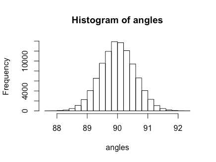
Note the scale of the x-axis: the angles are very closely bunched up around 90 degrees, as claimed.

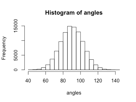
This phenomenon only happens for “high” dimensions. If we change the value of p above to 2, we obtain a very different histogram:

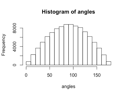
How “high” does the dimension have to be before we see this phenomenon kick in? Well, it depends on how tightly bunched up we want the angles to be around 90 degrees. The histogram below is the same simulation but for p = 20 (notice the wider x-axis scale):

It seems like the bell-shaped curve already starts to appear with p = 3!

Fact 2: Generate 10,000 random vectors in 20,000 dimensional space. Now, generate another random vector in that space. Then the angle between this vector and its projection on the span of the first 10,000 vectors is very likely to be very near 45 degrees.

Cook presents a very cool intuitive explanation of this fact which I highly recommend. Here, I present simulation evidence of the fact.

The difficulty in this simulation is computing the projection of a vector onto the span of many vectors. It can be shown that the projection of a vector onto the column span of a (full-rank) matrix is given by (see this post and this post for details). For our fact, is a matrix, so computing is going to take prohibitively long.

I don’t know another way to compute the projection of a vector onto the span of other vectors. (Does anyone know of better ways?) Fortunately, based on my simulations in Fact 1, this phenomenon will probably kick in for much smaller dimensions too!

First, let’s write up two functions: one that takes a vector v and matrix A and returns the projection of v onto the column span of A:

projectVec <- function(v, A) {
    A %*% solve(t(A) %*% A) %*% t(A) %*% v
}

and a function that does one run of the simulation. Here, p is the dimensionality of each of the vectors, and I assume that we are looking at the span of p/2 vectors:

simulationRun <- function(p) {
    A <- replicate(p/2, genRandomVec(p))
    v <- genRandomVec(p)
    proj_v <- projectVec(v, A)
    findAngle(proj_v, v)
}

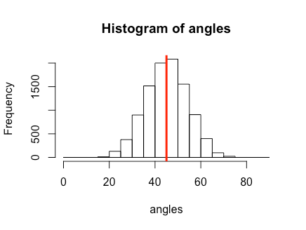
The code below runs 10,000 simulations for p = 20, taking about 2 seconds on my laptop:

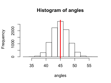
simN <- 10000 # no. of simulations
p <- 20     # dimension of the vectors
set.seed(54)
angles <- replicate(simN, simulationRun(p))
angles <- angles / pi * 180  # convert from radians to degrees
hist(angles, breaks = seq(0, 90, 5))
abline(v = 45, col = "red", lwd = 3)

We can already see the bunching around 45 degrees:

The simulation for p = 200 takes just under 2 minutes on my laptop, and we see tighter bunching around 45 degrees (note the x-axis scale).