
The End of the Honeymoon: Falling Out of Love with quantstrat
Want to share your content on R-bloggers? click here if you have a blog, or here if you don't.
Introduction
I spent good chunks of Friday, Saturday, and Sunday attempting to write another blog post on using R and the quantstrat package for backtesting, and all I have to show for my work is frustration. So I’ve started to fall out of love with quantstrat and am thinking of exploring Python backtesting libraries from now on.
Here’s my story…
Cross-Validation
Let’s suppose you’ve read my past blog posts on using R for analyzing stock data, in particular the most recent blog post on R for finance, on parameter optimization and order types. You’ll notice that we’ve been doing two things (perhaps among others):
- We only used most recent data as out-of-sample data. What if there are peculiarities unique to the most-recent time frame, and it’s not a good judge (alone) of future performance?
- We evaluate a strategy purely on its returns. Is this the best approach? What if a strategy doesn’t earn as much as another but it handles risk well?
I wanted to write an article focusing on addressing these points, by looking at cross-validation and different metrics for evaluating performance.
Data scientists want to fit training models to data that will do a good job of predicting future, out-of-sample data points. This is not done by finding the model that performs the best on the training data. This is called overfitting; a model may appear to perform well on training data but will not generalize to out-of-sample data. Techniques need to be applied to prevent against it.
A data scientist may first split her data set used for developing a predictive algorithm into a training set and a test set. The data scientist locks away the test set in a separate folder on the hard drive, never looking at it until she’s satisfied with the model she’s developed using the training data. The test set will be used once a final model has been found to determine the final model’s expected performance.
She would like to be able to simulate out-of-sample performance with the training set, though. The usual approach to do this is split the training set into, say, 10 different folds, or smaller data sets, so she can apply cross-validation. With cross-validation, she will choose one of the folds to be held out, and she fits a predictive model on the remaining nine folds. After fitting the model, she sees how the fitted model performs on the held-out fold, which the fitted model has not seen. She then repeats this model for the nine other folds, to get a sense of the distribution of the performance of the model, or average performance, on out-of-sample data. If there are hyperparameters (which are parameters that describe some higher-order aspect of a model and not learned from the data in the usual way other prarameters are; they’re difficult to define rigorously), she may try different combinations of them and see which combination lead to the model with the best predictive ability in cross-validation. After determining which predictive model generally leads to the best results and which hyperparameters lead to optimal results, she trains a model on the training set with those hyperparameters, evaluates its performance on the test set, and reports the results, perhaps deploying the model.
For those developing trading algorithms, the goals are similar, but there are some key differences:
- We evaluate a trading method not by predictive accuracy but by some other measure of performance, such as profitability or profitability relative to risk. (Maybe predictive accuracy is profitable, maybe not; if the most profitable trading system always underestimates its profitability, we’re fine with it.)
- We are using data where time and the order in which data comes in is thought to matter. We cannot just reshuffle data; important features would be lost. So we cannot divide up the data set randomly into different folds; order must be preserved.
I’ll talk more about how we could evaluate a trading system later; for now, let’s focus on how we can apply the idea of cross-validation analysis.
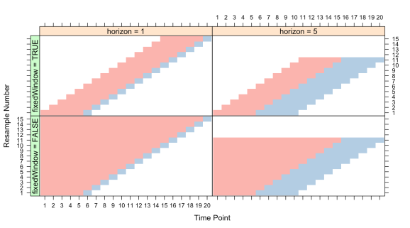
(Illustration by Max Kuhn in his book, The caret Package.)
For time-dependent data, we can employ walk-forward analysis or rolling forecast origin techniques. This comes in various flavors (see the above illustration), but I will focus on one flavor. We first divide up the data set into, say, ten periods. We first fit a trading algorithm on the first period in the data set, then see how it performs on the “out-of-sample” second period. Then we repeat for the second and third periods, third and fourth periods, and so on until we’ve run to the end of the data set. The out-of-sample data sets are then used for evaluating the potential performance of the trading system in question. If we like, we may be keeping a final data set, perhaps the most recent data set, for final evaluation of whatever trading system passes this initial test.
Other variants include overlapping training/testing periods (as described, my walk-forward analysis approach does not overlap) or ones where the initial window grows from beginning to end. Of these, I initially think either the approach I’ve described or the approach with overlapping training/testing periods makes most sense.
Attempting to Use quantstrat
I discovered that quantstrat has a function that I thought would implement the type of walk-forward analysis I wanted, called walk.forward(). I was able to define a training period duration, a testing period duration, an objective function to maximize, and many other features I wanted. It could take a strategy designed for optimization with apply.paramset() and apply a walk-forward analysis.
So I tried it once and the results were cryptic. The function returns a list with the results of training… but no sign of the test results. I would try looking at the portfolio object and tradeStats() output, but there was no sign of a portfolio. I had no idea why. I still have no idea where the portfolio went initially. I would try clearing my environments and restarting R and doing the whole process again. Same results: no sign of a portfolio, and all I got was a list of results for training data, with no sign of results for testing data. I looked at the source code. I saw that it was doing something with the test data: it was using applyStrategy() on the test data.
I had no idea what the hell that meant. When I use applyStrategy() as the user, I have to assume that the portfolio is wiped out, the account is reset, and every application is effectively a fresh start. So when I saw that line, it looked as if the function got an optimized function, applied it to the test data, and would repeat this process all the while forgetting the results of previous applications of the optimized strategy to test data sets. But online sources said that was not what was happening; the results of this backtesting were being appended back-to-back, which did not mesh with either my notion of walk-forward analysis (which allows for overlapping time frames, which does not mean you can “glue” together test data results) or what applyStrategy() does. And it still does not make sense to me. (That is what it does, though.)
The fact that the demonstration of walk.forward() supplied with quantstrat is bugged (and I never found how to fix all its bugs) didn’t help.
So I tried using the function’s auditing feature; by supplying a string to audit.prefix, *.RData files will be created containing the results of training and testing, storing them in a special .audit environment. So I changed the working directory to one specifically meant for the audit files (there could be a lot of them and I didn’t want to clutter up my other directories; I hate clutter), passed a string to audit.prefix, and tried again. After the analysis was completed, I look in the directory to see the files.
There’s nothing there.
It took hours and I had to go through a debugger to finally discover that walk.forward() was saving files, but it was using my Documents directory as the working directory, not the directory I setwd()ed into. Why? I have no idea. It could be quantstrat, blotter, or RStudio’s workbooks. I have no idea how long it took to figure out where my files had gone, but it was too long however long it was.
Good news though was that I now could try and figure out what was happening to the test data. This presentation by Guy Yollin was helpful, though it still took a while to get it figured out.
From what I can tell, what walk.forward() does is simulate a trading strategy that optimizes, trades, and re-optimizes on new data, and trades. So it doesn’t look like cross-validation as I described but rather a trading strategy, and that’s not really what I wanted here. I wanted to get a sense of the distribution of returns when using window sizes chosen optimally from backtesting. I don’t think there’s any simple way to do that with quantstrat.
Furthermore, I can’t see how I can collect the kind of statistics I want, such as a plot of the value of the account or the account’s growth since day one, with the way the walk-forward analysis is being done. Furthermore, the results I did get look… strange. I don’t know how those kinds of results would appear… at all. They look like nonsense. So I don’t even know if the function is working right.
Oh, did I mention that I discovered that the way I thought backtesting was being done isn’t how it’s actually done in quantstrat? When I was doing backtesting, I would rather see the results of the backtest on a variety of stocks instead of just one. I imagine an automated backtest behaving like a trader with an account, and active trades tie up the trader’s funds. So if the trader sees an opportunity but does not have the cash to act on it, the trader does not take the trade. (There is no margin here.)
I thought applyStrategy() was emulating such a trader, but the documentation (and the logs produced, for that matter), suggest that’s not what’s happening. It backtests on each symbol separately, unaware of any other positions that may exist. I don’t like that.
It was very difficult to figure this all out, especially given the state of the documentation currently. That said, in the developers’ defense, quantstrat is still considered under heavy development. Maybe in the future the documentation will be better. I feel, though, that creating good documentation is not something done once you’ve completed coding; you write good documentation as you code, not after.
blotter: The Fatal Flaw
Granted, I’m an ignorant person, but I don’t feel like all the confusion that lead to me wasting my weekend is completely my fault. quantstrat‘s design is strange and, honestly, not that intuitive. I think the problem stems from quantstrat‘s building off an older, key package: blotter.
blotter is a package intended to manage transactions, accounts, portfolios, financial instruments, and so on. All the functions for creating accounts and portfolios are blotter functions, not quantstrat functions. blotter does this by setting up its own environment, the .blotter environment, and the functions I’ve shown are for communicating with this environment, adding and working with entities stored in it.
I don’t know what the purpose of creating a separate environment for managing those objects is. I feel that by doing so a wall has been placed between me and the objects I’m trying to understand. quantstrat takes this further by defining a .strategy environment where strategies actually “live”, so we must use special functions to interact with that separate universe, adding features to our strategies, deleting and redefining them with special functions, and so on.
To me, this usage of environments feels very strange, and I think it makes quantstrat difficult and unintuitive. In some sense, I feel like strategies, portfolios, accounts, etc. are pseudo-objects in the object oriented programming (OOP) sense, and the developers of blotter and quantstrat are trying to program like R is a language that primarily follows the OOP paradigm.
While R does support OOP, it’s a very different kind of OOP and I would not call R an OOP language. R is a functional programming language. Many see the tidyverse as almost revolutionary in making R easy to use. That’s because the tidyverse of package, including ggplot2, magrittr, dplyr, and others, recognize that R relies on the functional programming paradigm and this paradigm does, in fact, lead to elegant code. Users can write pipelines and functions to put into pipelines that make complicated tasks easy to program. No part of the pipeline is cut off from the user, and the process of building the pipeline is very intuitive.
When I wrote my first blog post on R for finance and trading, one of the common comments I heard was, “tidyquant is better.” I have yet to look seriously at tidyquant, and maybe it is better, but so far all I’ve seen is tidyquant replace quantmod‘s functionality, and I have no complaint with quantmod (although tidyquant may also be suffering from the original sin of relying too heavily on environments). That said, the tidyquant approach may yet be the future of R backtesting.
Let’s try re-imagining what a better R backtesting package might look like, one that takes lessons from the tidyverse. Let’s first look at defining a strategy with quantstrat (after all the obnoxious boilerplate code).
portfolio_st <- "myStrat"

rm.strat(strategy_st)  # Must be done to delete or define a new strategy
strategy(strategy_st, store = TRUE)  # This is how to create a strategy

add.indicator(strategy = strategy_st, name = "SMA",
              arguments = list(x = quote(Cl(mktdata)),
                               n = 20),
              label = "fastMA")
add.indicator(strategy = strategy_st, name = "SMA",
              arguments = list(x = quote(Cl(mktdata)),
                               n = 50),
              label = "slowMA")

add.signal(strategy = strategy_st, name = "sigCrossover2",  # Remember me?
           arguments = list(columns = c("fastMA", "slowMA"),
                            relationship = "gt"),
           label = "bull")
add.signal(strategy = strategy_st, name = "sigCrossover2",
           arguments = list(columns = c("fastMA", "slowMA"),
                            relationship = "lt"),
           label = "bear")
add.rule(strategy = strategy_st, name = "ruleSignal",
         arguments = list(sigcol = "bull",
                          sigval = TRUE,
                          ordertype = "market",
                          orderside = "long",
                          replace = FALSE,
                          TxnFees = "fee",
                          prefer = "Open",
                          osFUN = osMaxDollarBatch,
                          maxSize = quote(floor(getEndEq(account_st,
                                                   Date = timestamp) * .1)),
                          tradeSize = quote(floor(getEndEq(account_st,
                                                   Date = timestamp) * .1)),
                          batchSize = 100),
         type = "enter", path.dep = TRUE, label = "buy")
add.rule(strategy = strategy_st, name = "ruleSignal",
         arguments = list(sigcol = "bear",
                          sigval = TRUE,
                          orderqty = "all",
                          ordertype = "market",
                          orderside = "long",
                          replace = FALSE,
                          TxnFees = "fee",
                          prefer = "Open"),
         type = "exit", path.dep = TRUE, label = "sell")
add.distribution(strategy_st,
                 paramset.label = "MA",
                 component.type = "indicator",
                 component.label = "fastMA",
                 variable = list(n = 5 * 1:10),
                 label = "nFAST")
add.distribution(strategy_st, paramset.label = "MA",
                 component.type = "indicator", component.label = "slowMA",
                 variable = list(n = 5 * 1:10), label = "nSLOW")
add.distribution.constraint(strategy_st,
                            paramset.label = "MA",
                            distribution.label.1 = "nFAST",
                            distribution.label.2 = "nSLOW",
                            operator = "<",
                            label = "MA.Constraint")
After all this code, we have a strategy that lives in the .strategy environment, locked away from us. What if we were to create strategies like we create plots in ggplot2? The code might look like this:
myStrat <- strategy() +
               indicator(SMA, args = list(x = Close, n = 20),
                         label = "fastMA") +
               indicator(SMA, args = list(x = Close, n = 50),
                         label = "slowMA") +
               signal(sigCrossover, quote(fastMA > slowMA), label = "bull") +
               signal(sigCrossover, quote(fastMA < slowMA), label = "bear") +
               rule( ..... ) +
               rule( ..... ) +
               distribution( ...... ) +
               distribution( ...... ) +
               distribution_constraint( ...... )
In blotter (and thus quantstrat) we create porfolios and accounts like so:
portfolio_st <- "myPortf"
account_st <- "myAcct"

rm.strat(portfolio_st)
rm.strat(account_st)
# This creates a portfolio
initPortf(portfolio_st, symbols = symbols,
          initDate = initDate, currency = "USD")
# Then an account
initAcct(account_st, portfolios = portfolio_st,
         initDate = initDate, currency = "USD",
         initEq = 100000)
# And finally an orderbook
initOrders(portfolio_st, store = TRUE)
Then we run the strategy with:
applyStrategy(strategy_st, portfolios = portfolio_st)
and we see the results with this code:
updatePortf(portfolio_st)
dateRange <- time(getPortfolio(portfolio_st)$summary)[-1]
updateAcct(account_st, dateRange)
updateEndEq(account_st)
tStats <- tradeStats(Portfolios = portfolio_st, use="trades",
                     inclZeroDays = FALSE)
tStats[, 4:ncol(tStats)] <- round(tStats[, 4:ncol(tStats)], 2)
print(data.frame(t(tStats[, -c(1,2)])))

final_acct <- getAccount(account_st)
plot(final_acct$summary$End.Eq["2010/2016"] / 100000,
     main = "Portfolio Equity", ylim = c(0.8, 2.5))
lines(SPY$SPY.Adjusted / SPY$SPY.Adjusted[[1]], col = "blue")
A tidyverse approach might look like the following:
# Create an account with a pipe
myAcct <- symbols %>%
            portfolio(currency = "USD") %>%
            account(currency = "USD", initEq = 100000)

# Backtesting generates an object containing the orderbook and all other
# necessary data (such as price at trade)
ob <- myAcct %>% myStrat  # This is a backtest
Other functions would then extract any information we need from the object ob, when we ask for them.
If I wanted to optimize, I might do the following:
ob_list <- myAcct %>% myStrat(optim = "MA")  # Gives a list of orderbooks, and
                                             # optimizes the parameter set MA
And as for the original reason I started to gripe, I might be able to find slices for the analysis with caret functions (they exist), subset the data in symbols according to these slices, and get ob in, say, an lapply() loop.
I like the idea for this interface, myself.
Conclusion (On To Python)
I do not have the time to write a package like this myself. I don’t know enough and I am a Ph.D. student and should be preparing for qualifying exams/research/etc.. For now, though, I’m turned off to quantstrat, and thus R for backtesting and trading.
That said, my stock data analysis posts are still, by far, the most popular content of this blog, and I still would like to find a good backtesting system. I’m looking at going back to Python, and the backtrader package has caught my eye. I will either use that or zipline, but I am leaning to backtrader, since initially I like its logging features and its use of OOP.
I would love to hear thoughts and comments, especially from users of either backtrader or zipline or Python for stock data analysis in general.

R-bloggers.com offers daily e-mail updates about R news and tutorials about learning R and many other topics. Click here if you're looking to post or find an R/data-science job.
Want to share your content on R-bloggers? click here if you have a blog, or here if you don't.