Introduction

With the drastic increase in the availability of text data on the web over the past decade, the field of Natural Language Processing has also had some great strides of advancement at an unprecedented rate. Like many topics in Machine Learning and AI, the rate of advancement in NLP is so fast that even methodologies that were state-of-the-art just a few of years ago is now considered obsolete. At the same time, because of the gain in popularity of NLP – among both corporations and professionals –  many open source tools have become available.

In this post, we will explore three of the most popular topics in Natural Language Processing: Sentiment Analysis, Word Embedding (also called Word2Vec), and Topic Modeling, using various open source tools in R.

Sentiment Analysis

Like many Machine Learning tasks, there are two major families of Sentiment Analysis: Supervised, and Unsupervised Learning.

In Supervised Sentiment Analysis, labeled sentences are used as training data to develop a model (e.g. “You like that movie” – Positive, “That movie was terrible” – Negative). Using labeled sentences, you train a machine learning model (methods range from as simple as Naive Bayes on unigrams, to Deep Recurrent Neural Networks with Word Embedding Layers and LSTM).

In Unsupervised Sentiment Analysis, labeled sentences are not required. Instead, they rely on lexicon of words with associated sentiment values. A simple lexicon would contain a dictionary of words with a classification of “positive” or “negative” (i.e. good = positive, bad = negative). Lexcions that are a little more sophisticated would have varying values assigned to different words (i.e. good = 0.5, great = 0.75).

While the Supervised method is generally known to have better performance, in this post we will explore the Unsupervised method (primarily due to not having the luxury of having pre-labeled sentences).

In this post, we will be working with reviews of the 2018 film Venom, scraped from Amazon.com. To find out how to scrape reviews from amazon, see this post.

First we’ll load the data.

# load packages for data cleaning and sentiment analysis
if(!"pacman" %in% installed.packages()[,"Package"]) install.packages("pacman")
pacman::p_load(dplyr)

# grab reviews
reviews_all = read.csv("https://raw.githubusercontent.com/rjsaito/Just-R-Things/master/NLP/sample_reviews_venom.csv", stringsAsFactors = F)

# create ID for reviews
review_df <- reviews_all %>%
  mutate(id = row_number())

str(reviews_all)

## 'data.frame':    1564 obs. of  8 variables:
##  $ prod         : chr  "Venom" "Venom" "Venom" "Venom" ...
##  $ title        : chr  "Large amounts of fun" "Nobody channels Eddie Brock / Venom like Tom Hardy. Nobody!" "What a stinker - easily the wost movie I have ever rented on Amazon and I deeply regret it." "Excellent!" ...
##  $ author       : chr  "MacJunegrand" "kiwijinxter" "Charles Schoch" "H. Tague" ...
##  $ date         : chr  "24-Oct-18" "12-Oct-18" "20-Dec-18" "11-Dec-18" ...
##  $ review_format: chr  "Format: Prime Video" "Format: Blu-ray" "Format: Prime VideoVerified Purchase" "Format: Prime VideoVerified Purchase" ...
##  $ stars        : int  5 5 1 5 1 1 1 1 5 5 ...
##  $ comments     : chr  "Movie critics have a though job, I get it. They have to watch lots of movies and not for pleasure, but as a job"| __truncated__ "As someone who had hundreds of Spider-Man comics when I was younger (I even owned a copy of Amazing Spider-Man "| __truncated__ "This movie was bad. How bad?  It is the only rental I have memory of where I deeply regret spending the 6 bucks"| __truncated__ "Been a huge fan of Venom since the 90s and been waiting for a good live action adaptation of him ever since and"| __truncated__ ...
##  $ n_helpful    : int  392 80 38 29 23 16 16 17 11 10 ...

This is a data.frame of 1,564 reviews of Venom on Amazon. It contains the product name (Venom), title of review, author, date, review format, star rating, comments, and # of customers who found the review helpful.

We will be performing a Lexicon-based Unsupervised Sentiment Analysis, using a package called sentimentr, written by Tyler Rinker. This lexicon based approach is in fact more sophisticated than it actually sounds, and takes into consideration concepts such as “amplifiers” and “valence shifters” when calculating the sentiment. The READ.me section of this gitub repo is worth a read if you are interested in learning what really happens under the hood.

We will load the package, and view the head of the default lexicon data frame to get a glimpse of what we will be working with.

# load packages for senitment analysis
pacman::p_load(tidyr, stringr, data.table, sentimentr, ggplot2)

# get n rows
nrow(lexicon::hash_sentiment_jockers_rinker)

## [1] 11710

# example lexicon
head(lexicon::hash_sentiment_jockers_rinker)

##              x     y
## 1:      a plus  1.00
## 2:     abandon -0.75
## 3:   abandoned -0.50
## 4:   abandoner -0.25
## 5: abandonment -0.25
## 6:    abandons -1.00

You can see that this default lexicon contains 11,710 words, each with a pre-assigned sentiment value. This is a rich lexicon to work with, but we will be making some modifications to this before we perform sentiment analysis on Venom. The reason we want to do this is, in the context of Venom, some words deserve a sentiment value from the one pre-assigned in the lexicon. An example is the word “Venom” itself – we know that in this film “Venom” refers to the main symbiote character, and thus should hold a neutral sentiment (i.e. sentiment = 0) as the sentiment will be determine by the words accompanying “Venom” rather than Venom itself. In the lexicon, the word “Venom” is assigned a value of -0.75, thus we will modify it to 0. While this step may be tedious, it is necessary in order to perform a more accurate, Domain Specific Sentiment Analysis.

Here are some other examples of words to modify in the lexicon.

# words to replace
replace_in_lexicon <- tribble(
  ~x, ~y,
  "marvel", 0,  # original score: .75
  "venom", 0,   # original score: -.75
  "alien", 0,   # original score: -.6
  "bad@$$", .4, # not in dictionary
  "carnage", 0, # original score: 0.75
  "avenger", 0, # original score: .25
  "riot", 0     # original score: -.5
)

# create a new lexicon with modified sentiment
venom_lexicon <- lexicon::hash_sentiment_jockers_rinker %>%
  filter(!x %in% replace_in_lexicon$x) %>%
  bind_rows(replace_in_lexicon) %>%
  setDT() %>%
  setkey("x")

Now that we have tailored the lexicon for Venom, we area ready to perform sentiment analysis. Using a combination of get_sentences() and sentiment_by(), we perform a sentence-level sentiment analysis:

# get sentence-level sentiment
sent_df <- review_df %>%
  get_sentences() %>%
  sentiment_by(by = c('id', 'author', 'date', 'stars', 'review_format'), polarity_dt = venom_lexicon)

After doing so, first let’s plot the sentiment by star rating, using a box plot. We would expect that the higher the star rating that a review has received, the higher the sentiment of the review.

# stars vs sentiment
p <- ggplot(sent_df, aes(x = stars, y = ave_sentiment, color = factor(stars), group = stars)) +
  geom_boxplot() +
  geom_hline(yintercept=0, linetype="dashed", color = "red") +
  geom_text(aes(5.2, -0.05, label = "Neutral Sentiment", vjust = 0), size = 3, color = "red") +
  guides(color = guide_legend(title="Star Rating")) +
  ylab("Avg. Sentiment") +
  xlab("Review Star Rating") +
  ggtitle("Sentiment of Venom Amazon Reviews, by Star Rating") 
p

You can see that is the case, with some variability. Furthermore, reviews with a star rating of 1 tend to be mostly consistently negative, while reviews with a star rating of 5 tends to be a mixed back of sentiment, while averaging high.

Let’s now plot the average sentiment over time.

# sentiment over time
sent_ts <- sent_df %>%
  mutate(
    date = as.Date(date, format = "%d-%B-%y"),
    dir = sign(ave_sentiment)
  ) %>%
  group_by(date) %>%
  summarise(
    avg_sent = mean(ave_sentiment)
  ) %>%
  ungroup()

# plot
p <- ggplot(sent_ts, aes(x = date, y = avg_sent)) +
  geom_smooth(method="loess", size=1, se=T, span = .6) +
  geom_vline(xintercept=as.Date("2018-10-05"), linetype="dashed", color = "black") +
  geom_text(aes(as.Date("2018-10-05") + 1, .4, label = "Theatrical Release", hjust = "left"), size = 3, color = "black") +
  geom_vline(xintercept=as.Date("2018-12-11"), linetype="dashed", color = "black") +
  geom_text(aes(as.Date("2018-12-11") + 1, .4, label = "Digital Release", hjust = "left"), size = 3, color = "black") +
  geom_vline(xintercept=as.Date("2018-12-18"), linetype="dashed", color = "black") +
  geom_text(aes(as.Date("2018-12-18") + 1, .37, label = "DVD / Blu-Ray Release", hjust = "left"), size = 3, color = "black") +
  geom_hline(yintercept=0, linetype="dashed", color = "red") +
  geom_text(aes(max(sent_ts$date) - 5, -0.02, label = "Neutral Sentiment", vjust = 0), size = 3, color = "red") +
  ylab("Avg. Sentiment") +
  xlab("Review Date") +
  ggtitle("Sentiment of Venom Amazon Reviews, Over Time (2018 - 2019)")
p

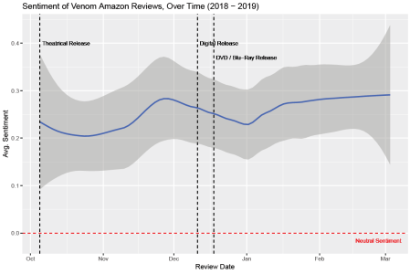
The sentiment for the film remained waekly positive over the course of the 5-month period, reaching an all time low towards the later half of October (few weeks into release), and a peak around the later half of November (Thanksgiving week).

Word Embeddings

Next, we will perform what is called Word Embedding (also known as word2vec. Word Embedding is a technique used to take a corpora (structured set of text, such as reviews), and transform it in such a way that it captures the context of a word in a document/review, its semantic and syntactic similarity, and its relation with other words. This is done by calculating a contexutal representation of a word in a vector form, and similar words will have vectors that are similar or close to each other, while words that are vasly different will be much further away.

There are many Word Embeddings methodology today, but the two most popular methods are:

1) Unsupervised learning on n-gram / dimensionality reduction on co-occurrence matrix, and
2) Skip gram model using Deep Neural Network

The latter requires time and resources (often requires GPU to train model in a reasonable amount of time), so in this post we will be exploring the former method. In specific, we will be using a method called GloVe (Global Vectors for Word Representation).

The package we will be using is called text2vec.

pacman::p_load(text2vec, tm, ggrepel)

The following code preprocesses the data, trains the model, and obtains the word vectors. To fully understand the algorithm for GloVe, this paper is a great reference – however using the default parameter settings is acceptable for most scenarios to start training your GloVe models.

Here are some consideration for the parameters, if you would like to tweak them:

• term_count_min: Minimum acceptable counts of a word in entire corpora to include in the model.
• skip_gram_window: The window size to search for a word-word co-occurence.
• word_vector_size: The length of the word embedding vector to train.
• x_max: A parameter in the cost function to adjust for co-word occurence (5 – 10 seems to be appropriate for small corpora)
• n_iter: # of training iterations to run (10 – 20 for small corpora).

# create lists of reviews split into individual words (iterator over tokens)
tokens <- space_tokenizer(reviews_all$comments %>%
                            tolower() %>%
                            removePunctuation())

# Create vocabulary. Terms will be unigrams (simple words).
it <- itoken(tokens, progressbar = FALSE)
vocab <- create_vocabulary(it)

# prune words that appear less than 3 times
vocab <- prune_vocabulary(vocab, term_count_min = 3L)

# Use our filtered vocabulary
vectorizer <- vocab_vectorizer(vocab)

# use skip gram window of 5 for context words
tcm <- create_tcm(it, vectorizer, skip_grams_window = 5L)

# fit the model. (It can take several minutes to fit!)
glove = GloVe$new(word_vectors_size = 100, vocabulary = vocab, x_max = 5)
glove$fit_transform(tcm, n_iter = 20)

# obtain word vector
word_vectors = glove$components

Now, using Brock‘s word vector, let’s see which words have the most contextual similarity (cosine similarity between word vectors):

brock <- word_vectors[, "brock", drop = F] 

cos_sim = sim2(x = t(word_vectors), y = t(brock), method = "cosine", norm = "l2")
head(sort(cos_sim[,1], decreasing = TRUE), 10)

##     brock     eddie   between     venom character        as  symbiote 
## 1.0000000 0.4668739 0.3277850 0.3141000 0.3071224 0.2868351 0.2769355 
##      both   someone     apart 
## 0.2613619 0.2497683 0.2465074

Contextually, (pro)nouns that are most similar to Brock is Eddie, Symbiote, Williams, Venom, Hardy (notice how Williams comes before Venom?).

Now using a popular visualization technique called t-SNE, which takes a high dimensional matrix, and converts it into a 2 or 3 dimensional representation of the data such that when plotted, similar objects appear nearby each other and dissimilar objects appear far away from each other.

# load packages
pacman::p_load(tm, Rtsne, tibble, tidytext, scales)

# create vector of words to keep, before applying tsne (i.e. remove stop words)
keep_words <- setdiff(colnames(word_vectors), stopwords())

# keep words in vector
word_vec <- word_vectors[, keep_words]

# prepare data frame to train
train_df <- data.frame(t(word_vec)) %>%
  rownames_to_column("word")

# train tsne for visualization
tsne <- Rtsne(train_df[,-1], dims = 2, perplexity = 50, verbose=TRUE, max_iter = 500)

## Performing PCA
## Read the 1391 x 50 data matrix successfully!
## OpenMP is working. 1 threads.
## Using no_dims = 2, perplexity = 50.000000, and theta = 0.500000
## Computing input similarities...
## Building tree...
## Done in 0.60 seconds (sparsity = 0.156655)!
## Learning embedding...
## Iteration 50: error is 66.664408 (50 iterations in 0.40 seconds)
## Iteration 100: error is 67.801968 (50 iterations in 0.41 seconds)
## Iteration 150: error is 67.846932 (50 iterations in 0.42 seconds)
## Iteration 200: error is 68.261359 (50 iterations in 0.41 seconds)
## Iteration 250: error is 67.974711 (50 iterations in 0.41 seconds)
## Iteration 300: error is 2.744975 (50 iterations in 0.30 seconds)
## Iteration 350: error is 2.694457 (50 iterations in 0.20 seconds)
## Iteration 400: error is 2.681063 (50 iterations in 0.21 seconds)
## Iteration 450: error is 2.669339 (50 iterations in 0.21 seconds)
## Iteration 500: error is 2.666172 (50 iterations in 0.21 seconds)
## Fitting performed in 3.17 seconds.

# create plot
colors = rainbow(length(unique(train_df$word)))
names(colors) = unique(train_df$word)

plot_df <- data.frame(tsne$Y) %>%
  mutate(
    word = train_df$word,
    col = colors[train_df$word]
  ) %>%
  left_join(vocab, by = c("word" = "term")) %>%
  filter(doc_count >= 20)

p <- ggplot(plot_df, aes(X1, X2)) +
  geom_text(aes(X1, X2, label = word, color = col), size = 3) +
  xlab("") + ylab("") +
  theme(legend.position = "none") 
p

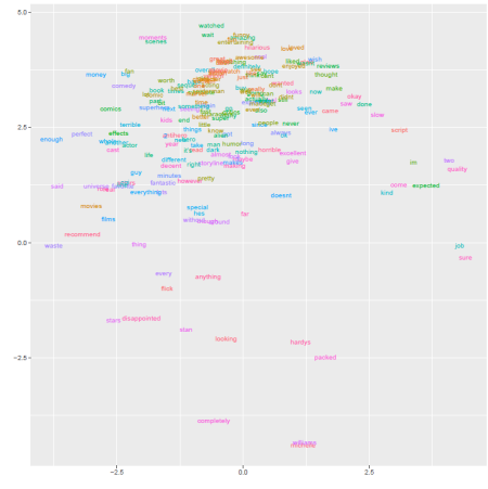
t-SNE maps high dimensional data such as word embedding into a lower dimension in such that the distance between two words roughly describe the similarity. Additionally it begins to create naturally forming clusters.

To make this even more interesting, let’s overlay sentiment. To estimate sentiment at the word level, we will use the sentence-level sentiment that we calculated before. To calcualte a word-level sentiment, we will simply take all the sentences that contain the word of interest, and take the average of sentiment across all thsoe sentences.

# calculate word-level sentiment
word_sent <- review_df %>%
  left_join(sent_df, by = "id") %>%
  select(id, comments, ave_sentiment) %>%
  unnest_tokens(word, comments) %>%
  group_by(word) %>%
  summarise(
    count = n(),
    avg_sentiment = mean(ave_sentiment),
    sum_sentiment = sum(ave_sentiment),
    sd_sentiment = sd(ave_sentiment)
  ) %>%
  # rtemove stop words
  anti_join(stop_words, by = "word") 

# filter to words that appear at least 5 times
pd_sent <- plot_df %>%
  left_join(word_sent, by = "word") %>%
  drop_na() %>%
  filter(count >= 5)

# create plot
p <- ggplot(pd_sent, aes(X1, X2)) +
  geom_point(aes(X1, X2, size = count, alpha = .1, color = avg_sentiment)) +
  geom_text(aes(X1, X2, label = word), size = 2) +
  scale_colour_gradient2(low = muted("red"), mid = "white",
                         high = muted("blue"), midpoint = 0) +
  scale_size(range = c(5, 20)) +
  xlab("") + ylab("") +
  ggtitle("2-dimensional t-SNE Mapping of Word Vectors") +
  guides(color = guide_legend(title="Avg. Sentiment"), size = guide_legend(title = "Frequency"), alpha = NULL) +
  scale_alpha(range = c(1, 1), guide = "none")
p

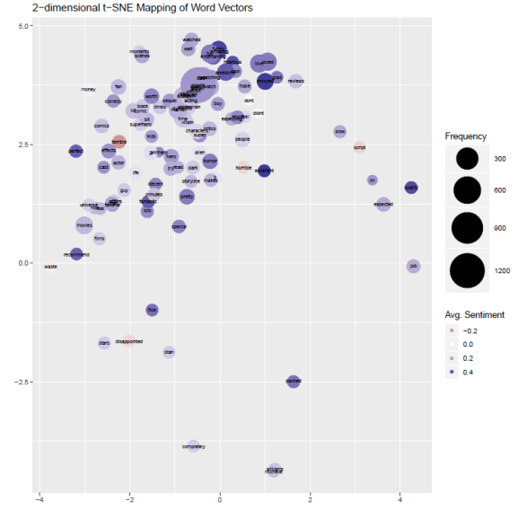
We have successfully plotted the frequency of word occurrence in the reviews, mapped the contextual word similarities using Word Embeddings, and overlaid the word-level sentiment by color.

Topic Modeling

The last method we will apply in this post is Topic Modeling. A Topic Model is a language learning model that identifies “topics”, in which words sharing similar contextual meanings appear together. It’s as if similar words are clustered together, except that a word can appear in multiple topics. Additionally, each document/review can be characterized by a single or multiple topics.

Topics are identified based on the detection of the likelihood of term co-occurrence, determined by a model. One of the most popular Topic Model today is called Latent Dirchlet Allocation, and as such, we will be using LDA for this post.

We will be using packages topicmodels and ldatuning for topic modeling using LDA, with help from tm and tidytext for data cleansing. First, we will remove any words that occur in less than 1% of the reviews.

# load packages
pacman::p_load(tm, topicmodels, tidytext, ldatuning)

# remove words that show up in more than 5% of documents
frequent_words <- vocab %>%
  filter(doc_count >= nrow(review_df) * .01) %>%
  rename(word = term) %>%
  select(word)

We will then be converting the reviews (or documents) into a Document Term Matrix (DTM). A DTM (or TDM for Term Document Matrix) is a very popular method of storing or structuring text data that allows for easy manipulation to do things such as calculate the TF-IDF (Term Frequency – Inverse Document Frequecy), or in this case, perform a Latent Dirchlet Allocation model.

# split into words
by_review_word <- reviews_all %>%
  mutate(id = 1:nrow(.)) %>%
  unnest_tokens(word, comments)

# find document-word counts
word_counts <- by_review_word %>%
  anti_join(stop_words, by = "word") %>%
  count(id, word, sort = TRUE) %>%
  ungroup()

dtm <- word_counts %>%
  cast_dtm(id, word, n)

To find the right number of topics, we run Latent Dirchlet Allocation at varying levels of k (# of topics), and determine the most appropriate number of topics by looking at several evaluation metrics.

# find topics
result <- FindTopicsNumber(
  dtm,
  topics = seq(from = 2, to = 15, by = 1),
  metrics = c("Griffiths2004", "CaoJuan2009", "Arun2010", "Deveaud2014"),
  method = "Gibbs",
  control = list(seed = 77),
  mc.cores = 2L,
  verbose = TRUE
)

## fit models... done.
## calculate metrics:
##   Griffiths2004... done.
##   CaoJuan2009... done.
##   Arun2010... done.
##   Deveaud2014... done.

FindTopicsNumber_plot(result)

By inspecting the “maximize” and “minimize” evaluation metrics, k = 6 topics seem to be an appropriate number.

We will now refit the model using k = 6, and within each topic return the top 20 words based on its beta value (which roughly represents how ‘informative’ the word is to the topic).

# set a seed so that the output of the model is predictable
my_lda <- topicmodels::LDA(dtm, k = 6, method = "Gibbs")

# transform into tidy data frame
ap_topics <- tidy(my_lda, matrix = "beta")

# for each topic, obtain the top 20 words by beta
pd <- ap_topics %>%
  group_by(topic) %>%
  top_n(20, beta) %>%  # top words based on informativeness
  ungroup() %>%
  arrange(topic, beta) %>%
  mutate(order = row_number()) 

# plot
ggplot(pd, aes(order, beta, fill = factor(topic))) +
  geom_col(show.legend = FALSE) +
  facet_wrap(~ topic, scales = "free") +
  # Add categories to axis
  scale_x_continuous(
    breaks = pd$order,
    labels = pd$term,
    expand = c(0,0)
  ) +
  coord_flip()

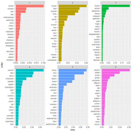
The topics that surface will be purely based on what the algorithm determines to be a common theme among the documents on which the model is trained, but once the topics are determined, we can label them according to the contextual similarity in the words that surface for each topic. For example, topic 1 seems to have a positive theme about the reception of the movie, while topic 2 has a negative tonality about the reception of the movie. Topic 4 seems to represent the plot, character, and comic of the Venomverse, and topic 6 is clearly the “Symbrock” topic.

And for the final viz, we will overlay the sentiment and the word vectors to create a single cohesive visualization that encapsulates all three Natural Language Processing tasks from this post.

# combine sentiment
pd_sent_topic <- pd_sent %>%
  left_join(ap_topics, by = c("word" = "term")) %>%
  filter(beta > .005) 
# create plot
p <- ggplot() +
  geom_point(data = pd_sent_topic, aes(X1, X2, size = count, alpha = .01, color = avg_sentiment)) +
  geom_text(data = pd_sent_topic, aes(X1, X2, label = word), size = 2) +
  scale_colour_gradient2(low = muted("red"), mid = "white",
                         high = muted("blue"), midpoint = 0) +
  scale_size(range = c(5, 20)) +
  xlab("") + ylab("") +
  ggtitle("2-dimensional t-SNE Mapping of Word Vectors") +
  guides(color = guide_legend(title="Sentiment"), size = guide_legend(title = "Frequency"), alpha = NULL) +
  scale_alpha(range = c(1, 1), guide = "none") +
  facet_wrap(~topic, scales=  "free")
p

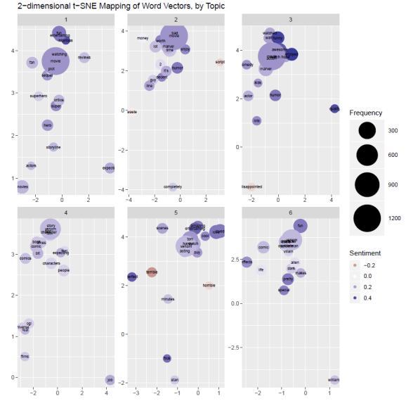
And voila. We have successfully created a single visualization that encapsulates the Sentiment (using Lexicon-based Domain-specific Sentiment Analysis), the Semantic Word Similarity (using GloVe Word Embedding), and the Topics (using Topic Modeling with Latent Dirichlet Allocation). I will add one note that, the performance of various Natural Language Processing will improve many folds with more and more text data, so it is recommended that you chase down and work with a large corpora of texts, rather than spend time tweaking the parameters to get them right.

If you found this post informative, please hit Subscribe or leave a comment!