
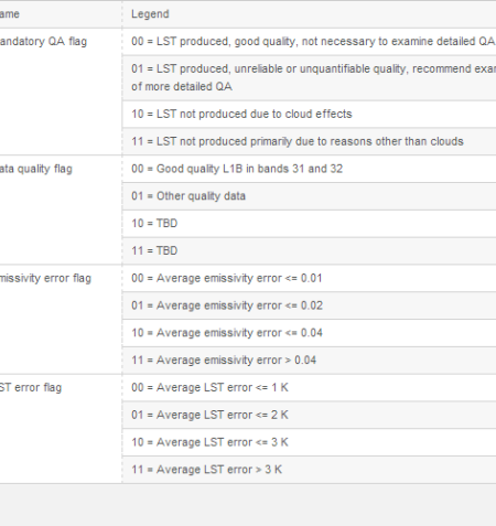
Modis QC Bits
Want to share your content on R-bloggers? click here if you have a blog, or here if you don't.
In the course of working through my MODIS LST project and reviewing the steps that Imhoff and Zhang took as well has the data preparations other researchers have taken ( Neteler ) the issue of MODIS Quality control bits came up. Every MODIS HDF file comes with multiple SDS or multiple layers of data. For MOD11A1 there are layers for daytime LST, Night LST, the time of collection, the emissivity from ch 31 and 32, and two layer for Quality Bits. The various layers of MODIS11A1 file is available here. Or if you are running the MODIS package, you can issue the getSds() call and pass it the name of a HDF file.
As Neteler notes the final LST files contain pixels of various quality. Pixels that are obscured by clouds are not produced, of course, but that does not entail that every pixel in the map is of the same quality. The SDS layers for QC – QC_day and QC_Night– contain the QC bits for every lat/lon in the LST map. On the surface this seem pretty straighforward, but deciding the bits can be a bit of a challenge. To do that I considered several source.
2. The Modis groups user guide
4. LP DAAC Tools, specifically the LDope tools provided by guys at MODLAN
I will start with 4, the ldope tools, If you are a hard core developer I think these tools would be a great addition to your bag of tricks. I won’t go into a lot of detail, but the tools allow you to do a host of processing on HDF files using a command line type interface. They provide source code in c and at some point in the future I expect that I would want to either write an R interface to these various tools or take the C code directly and wrap it in R. Since they have the code for reading HDF directly and quickly it might be a source to use to support the direct import of HDF into raster. However, I found nothing to really help with understanding the issue of decoding the QC bits. You can manipulate the QC layer and do a count of the various flags in the data set. Using the following command on all the tiles for the US I was able to poke around and figure out what flags are typically reported
comp_sds_values -sds=QC_Day C:\\Users\\steve\\Documents\\MODIS_ARC\\MODIS\\MOD11A1.005\\2005.07.01\\MOD11A1.A2005182.h08v05.005.2008040085443.hdf
However, I could do the same thing simply by loading a version of the whole US into raster and using the freq() command on raster. Figuring about what values are in the QC file is easy, but we want to understand what they mean. Let’s begin with that list of values. By looking at the frequency count of the US raster and by looking at a large collection of HDf files I found the following values for the QC layer
values <-c(0,2,3,5,17,21,65,69,81,85,129,133,145,149,193)
The question is what do they mean. The easiest one to understand is 0. A zero means that this pixel is highest quality. If we want only the highest quality pixels, then we can use the QC map, turn it into a logical mask and apply it to the LST map such that we only keep pixels that have 0 for their quality bits. There, job done!
Not so fast. We throw away many good pixels that way. To understand the QC bits lets start with the table provided
If you are not clear on how this works every number, every integer in the QC map is an unsigned 8 bit integer. The range of numbers is 0 to 255. The integers represent bit codes which requires you to do some base 2 math. That is not the tricky part. The number 8 for example would be “0001″ and 9 would be 1001. If you are unclear about binary representations of integers I suppose google is your friend.
Given the binary representation of the integer value we are then in a position to understand what the quality bits represent, but there is a minor complication which I’ll explain using an example. Let’s take the integer value of 65. In R the way we turn this into a binary representation is by using the call intToBits.
intToBits(65)
[1] 01 00 00 00 00 00 01 00 00 00 00 00 00 00 00 00 00 00 00 00 00 00 00 00
[25] 00 00 00 00 00 00 00 00
We only need 8 bits, so we should do the following
> intToBits(65)[1:8]
[1] 01 00 00 00 00 00 01 00
and for more clarity I will turn this into 0 and 1 like so
> as.integer(intToBits(65)[1:8])
[1] 1 0 0 0 0 0 1 0
So the first bit ( or bit 0 ) has a value of 1, and seventh bit ( bit 6 ) has a value of 1. We can check our math 2^6 =64 and 2^0 = 1, so it checks. Don’t forget that the 8 bits are numbered 0 to 7 and each represents a power of 2.
If you try to use this bit representation to understand the QC “state”, you will go horribly wrong!. It’s wrong because HDF files are written in big endian format. If you are not familiar with that, what you need to understand is that the least significant bit is on the right. In the example above the zero bit is on the left, so we need to flip the bits so that bit zero is on the right . Little Endian goes from right to left, 2^0 to 2^7. Big Endian goes left to right 2^7 to 2^0.
Little Endian: 1 0 0 0 0 0 1 0 = 65 2^0 + 2^6
Big Endian 0 1 0 0 0 0 0 1 = 65 2^6 + 2^0
The difference is this:
If we took 1 0 0 0 0 0 1 0 and ran it through the table, the table would indicate that the first two bits 10 would mean the pixel was not generated, and bit 1 in the 6th position would indicate an LST error of <= 3K. Now flip those bits
> f<-as.integer(intToBits(65)[1:8])
> f[8:1]
[1] 0 1 0 0 0 0 0 1
This bit order has the first two bits as 01 which indicates that the pixel is produced, but that other quality bits should be checked. Since bit 6 is 1 that indicates the pixel has an error > 2Kelvin but less than 3K
In short, to understand the QC bits we first turn the integer into a bit notation and then we flip the order of the bits and then use the table to figure out the QC status. For MOD11A1 I wrote a quick little program to generate all the possible bits and then add descriptive fields. I would probably do this for every Modis project I worked on especially since I dont work in binary everyday and I made about 100 mistakes trying to do this in my head.
QC_Data <- data.frame(Integer_Value = 0:255,
Bit7 = NA,
Bit6 = NA,
Bit5 = NA,
Bit4 = NA,
Bit3 = NA,
Bit2 = NA,
Bit1 = NA,
Bit0 = NA,
QA_word1 = NA,
QA_word2 = NA,
QA_word3 = NA,
QA_word4 = NA
)
for(i in QC_Data$Integer_Value){
AsInt <- as.integer(intToBits(i)[1:8])
QC_Data[i+1,2:9]<- AsInt[8:1]
}
QC_Data$QA_word1[QC_Data$Bit1 == 0 & QC_Data$Bit0==0] <- “LST GOOD”
QC_Data$QA_word1[QC_Data$Bit1 == 0 & QC_Data$Bit0==1] <- “LST Produced,Other Quality”
QC_Data$QA_word1[QC_Data$Bit1 == 1 & QC_Data$Bit0==0] <- “No Pixel,clouds”
QC_Data$QA_word1[QC_Data$Bit1 == 1 & QC_Data$Bit0==1] <- “No Pixel, Other QA”
QC_Data$QA_word2[QC_Data$Bit3 == 0 & QC_Data$Bit2==0] <- “Good Data”
QC_Data$QA_word2[QC_Data$Bit3 == 0 & QC_Data$Bit2==1] <- “Other Quality”
QC_Data$QA_word2[QC_Data$Bit3 == 1 & QC_Data$Bit2==0] <- “TBD”
QC_Data$QA_word2[QC_Data$Bit3 == 1 & QC_Data$Bit2==1] <- “TBD”
QC_Data$QA_word3[QC_Data$Bit5 == 0 & QC_Data$Bit4==0] <- “Emiss Error <= .01″
QC_Data$QA_word3[QC_Data$Bit5 == 0 & QC_Data$Bit4==1] <- “Emiss Err >.01 <=.02″
QC_Data$QA_word3[QC_Data$Bit5 == 1 & QC_Data$Bit4==0] <- “Emiss Err >.02 <=.04″
QC_Data$QA_word3[QC_Data$Bit5 == 1 & QC_Data$Bit4==1] <- “Emiss Err > .04″
QC_Data$QA_word4[QC_Data$Bit7 == 0 & QC_Data$Bit6==0] <- “LST Err <= 1″
QC_Data$QA_word4[QC_Data$Bit7 == 0 & QC_Data$Bit6==1] <- “LST Err > 2 LST Err <= 3″
QC_Data$QA_word4[QC_Data$Bit7 == 1 & QC_Data$Bit6==0] <- “LST Err > 1 LST Err <= 2″
QC_Data$QA_word4[QC_Data$Bit7 == 1 & QC_Data$Bit6==1] <- “LST Err > 4″
Which looks like this

Next, I will remove those flags that don’t matter. All good pixels, all pixels that don’t get drawn, and those where the TBD bit is set high. What I want to do is select all those flags where the pixel is produced but the pxel quality is not the highest quality
FINAL <- QC_Data[QC_Data$Bit1 == 0 & QC_Data$Bit0 ==1 & QC_Data$Bit3 !=1,]. Below see a part of this table

And then I can select those that occur in my HDF files.

Looking at LST error which matters most to me, the table indicates that I can use pixels that have a QC value of 0,5,17 and 21. I want to only select pixels where LSt error is less than 1 K
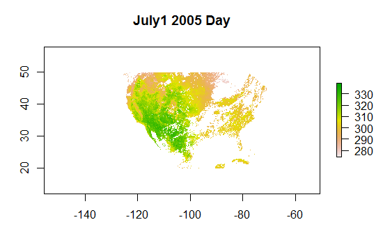
Very quickly I’ll show how one uses raster functions to apply the QC bits to LST. using MODIS R and the function getHdf() I’ve downloaded all the tiles for US for every day in July 2005. For July 1st, I’ve used MRT to mosiac and resample all the SDS. I use Nearest neighbor to insure that I dont average quality bits. The mosaic is the projected from a SIN projection to a Geographic projection ( WGS84) and a geotiff output format. Pixel size is set at 30 arc seconds
The SDS are read in using R’s raster
library(raster)
## get every layer of data in the July1 directory
SDS <- list.files(choose.dir(),full.names=T)
## for now I just work with the Day data
DayLst <- raster(SDS[7])
DayQC <- raster(SDS[11])
## The fill value for LST is Zero. That means Zero represents a No Data pixel
## So, we force those pixels to NA
DayLst[DayLst==0]<-NA
NightLst[NightLst==0]<-NA
## Units in LST need to be scaled to be put into Kelvin. The adjustment value is .02. See the docs for these values
## every SDS has a different fill value and a different scaling value.
DayLst <- DayLst * .02
Now, we can plot the two raster
plot(DayLst, main = “July1 2005 Day”)
plot(DayQC, main=”Day Quality COntrol”)
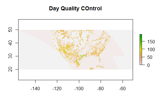
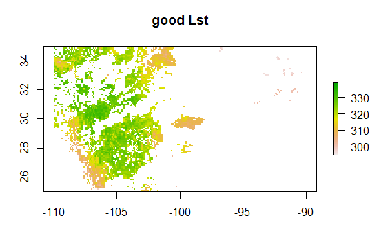
And I note that the area around texas has a nice variety of QC bits, so we can zoom in on that


Next we will use the QC layer and create mask
m <- DayQC
m[m > 21]<-NA
m[ m == 2 | m== 3]<-NA
Good <- mask(DayLst, m)
For this mask I’ve set all those grids with QC bits greater than 21 to NA. I’ve also set QC pixels with a value of 2 and 3 to NA. This step isnt really necessary since QC values of 2 and 3 mean that the pixel doesnt get produce, but I want to draw a map of the mask which will show which bits are NA and which bits are not NA. The mask() function works like so. “m” is laid over DayLst. bits that are NA in “m” will be NA in the destination (“Good”) if a pixel is not NA in “m” and has a value like, 0 or 17 or 25, then the value of the source (DayLst) is written into the destination.
Here are the values in my mask
> freq(m)
value count
[1,] 0 255179
[2,] 5 12
[3,] 17 8539
[4,] 21 3
[5,] NA 189147
So the mask will “block” 189147 pixels in DayLst from being copied from source to destination, while allowing the source pixels that have QC bits of 0,5,17,21 to be written. These QC bits are those that represent an LST error of less than 1K

When this mask is applied the colored pixels will be replaced by the values in the “source”
And to recall, these are all the pixels PRIOR to the application of the QC bits
As a side note, one thing I noticed when doing my SUHI analysis was that the LST data had a large variance over small areas. Even when I normalized for elevation and slope and land class there were pixels that were 10+ Kelvin warmer than the means. Essentially 6 sigma cases. That, of course lead me to have a look at the QC bits. Hopefully, this will improve some of the R^2 I was getting in my test regressions.

R-bloggers.com offers daily e-mail updates about R news and tutorials about learning R and many other topics. Click here if you're looking to post or find an R/data-science job.
Want to share your content on R-bloggers? click here if you have a blog, or here if you don't.