
Mapping Biodiversity data on smaller than one degree scale
Want to share your content on R-bloggers? click here if you have a blog, or here if you don't.
Guest Post by Enjie (Jane) LI
I have been using bdvis package (version 0.2.9) to visualize the iNaturalist records of RAScals project (http://www.inaturalist.org/projects/rascals).
Initially, the mapgrid function in the bdvis version 0.2.9 was written to map the number of records, number of species and completeness in a 1-degree cell grid (~111km x 111km resolution).
I applied this function to the RASCals dataset, see the following code. However, the mapping results are not satisfying. The 1 degree cells are too big to reveal the details in the study areas. Also, the raster grid was on top the basemap, which makes it really hard to associate the mapping results with physical locations.
library(rinat)
library(bdvis)

rascals=get_inat_obs_project("rascals")
conf <- list(Latitude="latitude",
             Longitude="longitude",
             Date_collected="Observed.on",
             Scientific_name="Scientific.name")
rascals <- format_bdvis(rascals, config=conf)
## Get rid of a record with weird location log
rascals <- rascals[!(rascals$Id== 4657868),]
rascals <- getcellid(rascals)
rascals <- gettaxo(rascals)
bdsummary(rascals)

a <- mapgrid(indf = rascals, ptype = "records",
             title = "distribution of RASCals records",
             bbox = NA, legscale = 0, collow = "blue",
             colhigh = "red", mapdatabase = "county",
             region = "CA", customize = NULL)

b <- mapgrid(indf = rascals, ptype = "species",
              title = "distribution of species richness of RASCals records",
              bbox = NA, legscale = 0, collow = "blue",
              colhigh = "red", mapdatabase = "county",
              region = "CA", customize = NULL)
I contacted developers of the package regarding these two issues. They have been very responsive to resolve them. They quickly added the gridscale argument in the mapgrid function. This new argument allows the users to choose scale (0.1 or 1). The default 1-degree cell grid for mapping.
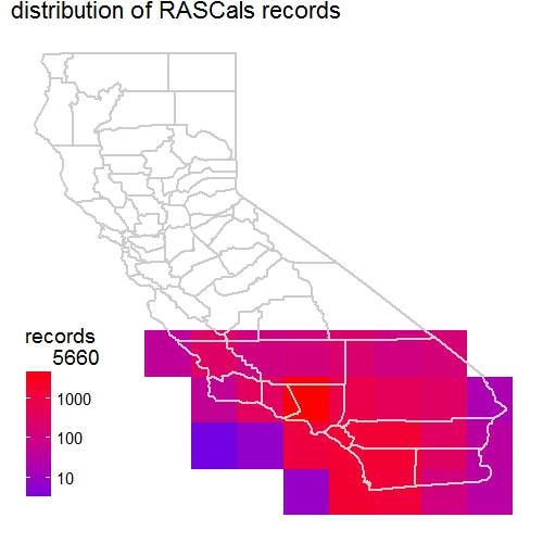
Here are mapping results from using the gridscale argument. Make sure you have bdvis version 0.2.14 or later.
c <- mapgrid(indf = rascals, ptype = "records",
title = "distribution of RASCals records",
bbox = NA, legscale = 0, collow = "blue",
colhigh = "red", mapdatabase = "county",
region = "CA", customize = NULL,
gridscale = 0.1)
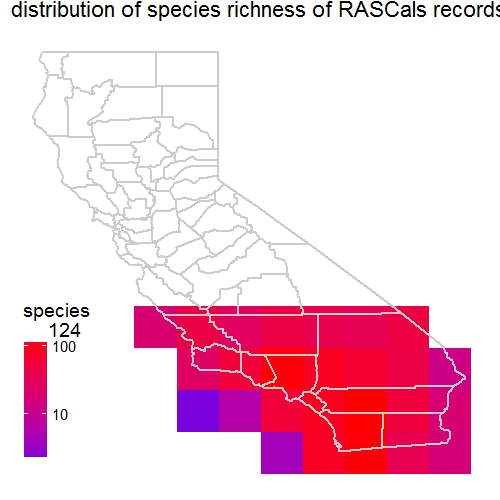
d <- mapgrid(indf = rascals, ptype = "species",
title = "distribution of species richness of RASCals records",
bbox = NA, legscale = 0, collow = "blue",
colhigh = "red", mapdatabase = "county",
region = "CA", customize = NULL,
gridscale = 0.1)


We can see that the new map with a finer resolution definitely revealed more information within the range of our study area. One more thing to note is that in this version developers have adjusted the basemap to be on top of the raster layer. This has definitely made the map easier to read and reference back to the physical space.
Good job team! Thanks for developing and perfecting the bdvis package.
References
- RASCals: http://www.inaturalist.org/projects/rascals
- Barve, V., & Otegui, J. (2016). bdvis: Biodiversity data visualizations Version: 0.2.9 Accessed from https://cran.r-project.org/web/packages/bdvis/index.html
- Barve, V., & Otegui, J. (2017). bdvis: Biodiversity data visualizations Version: 0.2.14 Accessed from https://github.com/vijaybarve/bdvis

R-bloggers.com offers daily e-mail updates about R news and tutorials about learning R and many other topics. Click here if you're looking to post or find an R/data-science job.
Want to share your content on R-bloggers? click here if you have a blog, or here if you don't.