This post will display some robustness results for KDA asset allocation.

Ultimately, the two canary instruments fare much better using the original filter weights in Defensive Asset Allocation than in other variants of the weights for the filter. While this isn’t as worrying (the filter most likely was created that way and paired with those instruments by design), what *is* somewhat more irritating is that the strategy is dependent upon the end-of-month phenomenon, meaning this strategy cannot be simply tranched throughout an entire trading month.

So first off, let’s review the code from last time:

# KDA asset allocation 
# KDA stands for Kipnis Defensive Adaptive (Asset Allocation).

# compute strategy statistics
stratStats <- function(rets) {
  stats <- rbind(table.AnnualizedReturns(rets), maxDrawdown(rets))
  stats[5,] <- stats[1,]/stats[4,]
  stats[6,] <- stats[1,]/UlcerIndex(rets)
  rownames(stats)[4] <- "Worst Drawdown"
  rownames(stats)[5] <- "Calmar Ratio"
  rownames(stats)[6] <- "Ulcer Performance Index"
  return(stats)
}

# required libraries
require(quantmod)
require(PerformanceAnalytics)
require(tseries)

# symbols
symbols <- c("SPY", "VGK",   "EWJ",  "EEM",  "VNQ",  "RWX",  "IEF",  "TLT",  "DBC",  "GLD", "VWO", "BND")  


# get data
rets <- list()
for(i in 1:length(symbols)) {
  
  returns <- Return.calculate(Ad(get(getSymbols(symbols[i], from = '1990-01-01'))))
  colnames(returns) <- symbols[i]
  rets[[i]] <- returns
}
rets <- na.omit(do.call(cbind, rets))


# algorithm
KDA <- function(rets, offset = 0, leverageFactor = 1.5, momWeights = c(12, 4, 2, 1)) {
  
  # get monthly endpoints, allow for offsetting ala AllocateSmartly/Newfound Research
  ep <- endpoints(rets) + offset
  ep[ep < 1] <- 1
  ep[ep > nrow(rets)] <- nrow(rets)
  ep <- unique(ep)
  epDiff <- diff(ep)
  if(last(epDiff)==1) { # if the last period only has one observation, remove it
    ep <- ep[-length(ep)]
  }
  
  # initialize vector holding zeroes for assets
  emptyVec <- data.frame(t(rep(0, 10)))
  colnames(emptyVec) <- symbols[1:10]
  
  
  allWts <- list()
  # we will use the 13612F filter
  for(i in 1:(length(ep)-12)) {
    
    # 12 assets for returns -- 2 of which are our crash protection assets
    retSubset <- rets[c((ep[i]+1):ep[(i+12)]),]
    epSub <- ep[i:(i+12)]
    sixMonths <- rets[(epSub[7]+1):epSub[13],]
    threeMonths <- rets[(epSub[10]+1):epSub[13],]
    oneMonth <- rets[(epSub[12]+1):epSub[13],]
    
    # computer 13612 fast momentum
    moms <- Return.cumulative(oneMonth) * momWeights[1] + Return.cumulative(threeMonths) * momWeights[2] + 
      Return.cumulative(sixMonths) * momWeights[3] + Return.cumulative(retSubset) * momWeights[4]
    assetMoms <- moms[,1:10] # Adaptive Asset Allocation investable universe
    cpMoms <- moms[,11:12] # VWO and BND from Defensive Asset Allocation
    
    # find qualifying assets
    highRankAssets <- rank(assetMoms) >= 6 # top 5 assets
    posReturnAssets <- assetMoms > 0 # positive momentum assets
    selectedAssets <- highRankAssets & posReturnAssets # intersection of the above
    
    # perform mean-variance/quadratic optimization
    investedAssets <- emptyVec
    if(sum(selectedAssets)==0) {
      investedAssets <- emptyVec
    } else if(sum(selectedAssets)==1) {
      investedAssets <- emptyVec + selectedAssets 
    } else {
      idx <- which(selectedAssets)
      # use 1-3-6-12 fast correlation average to match with momentum filter  
      cors <- (cor(oneMonth[,idx]) * momWeights[1] + cor(threeMonths[,idx]) * momWeights[2] + 
                 cor(sixMonths[,idx]) * momWeights[3] + cor(retSubset[,idx]) * momWeights[4])/sum(momWeights)
      vols <- StdDev(oneMonth[,idx]) # use last month of data for volatility computation from AAA
      covs <- t(vols) %*% vols * cors
      
      # do standard min vol optimization
      minVolRets <- t(matrix(rep(1, sum(selectedAssets))))
      minVolWt <- portfolio.optim(x=minVolRets, covmat = covs)$pw
      names(minVolWt) <- colnames(covs)
      investedAssets <- emptyVec
      investedAssets[,selectedAssets] <- minVolWt
    }
    
    # crash protection -- between aggressive allocation and crash protection allocation
    pctAggressive <- mean(cpMoms > 0)
    investedAssets <- investedAssets * pctAggressive 
    
    pctCp <- 1-pctAggressive
    
    # if IEF momentum is positive, invest all crash protection allocation into it
    # otherwise stay in cash for crash allocation
    if(assetMoms["IEF"] > 0) {
      investedAssets["IEF"] <- investedAssets["IEF"] + pctCp
    }
    
    # leverage portfolio if desired in cases when both risk indicator assets have positive momentum
    if(pctAggressive == 1) {
      investedAssets = investedAssets * leverageFactor
    }
    
    # append to list of monthly allocations
    wts <- xts(investedAssets, order.by=last(index(retSubset)))
    allWts[[i]] <- wts
    
  }
  
  # put all weights together and compute cash allocation
  allWts <- do.call(rbind, allWts)
  allWts$CASH <- 1-rowSums(allWts)
  
  # add cash returns to universe of investments
  investedRets <- rets[,1:10]
  investedRets$CASH <- 0
  
  # compute portfolio returns
  out <- Return.portfolio(R = investedRets, weights = allWts)
  return(list(allWts, out))
}

So, the idea is that we take the basic Adaptive Asset Allocation algorithm, and wrap it in a canary universe from Defensive Asset Allocation (see previous post for links to both), which we use to control capital allocation, ranging from 0 to 1 (or beyond, in cases where leverage applies).

One of the ideas was to test out different permutations of the parameters belonging to the canary filter–a 1, 3, 6, 12 weighted filter focusing on the first month.

There are two interesting variants of this–equal weighting on the filter (both for momentum and the safety assets), and reversing the weights (that is, 1 * 1, 3 * 2, 6 * 4, 12 * 12). Here are the results of that experiment:

# different leverages
KDA_100 <- KDA(rets, leverageFactor = 1)
KDA_EW <- KDA(rets, leverageFactor = 1, momWeights = c(1,1,1,1))
KDA_rev <- KDA(rets, leverageFactor = 1, momWeights = c(1, 2, 4, 12))
# KDA_150 <- KDA(rets, leverageFactor = 1.5)
# KDA_200 <- KDA(rets, leverageFactor = 2)

# compare
compare <- na.omit(cbind(KDA_100[[2]], KDA_EW[[2]], KDA_rev[[2]]))
colnames(compare) <- c("KDA_base", "KDA_EW", "KDA_rev")
charts.PerformanceSummary(compare, colorset = c('black', 'purple', 'gold'), 
                          main = "KDA AA with various momentum weights")

stratStats(compare)
apply.yearly(compare, Return.cumulative)

With the following results:

> stratStats(compare)
                            KDA_base    KDA_EW   KDA_rev
Annualized Return         0.10990000 0.0879000 0.0859000
Annualized Std Dev        0.09070000 0.0900000 0.0875000
Annualized Sharpe (Rf=0%) 1.21180000 0.9764000 0.9814000
Worst Drawdown            0.07920363 0.1360625 0.1500333
Calmar Ratio              1.38756275 0.6460266 0.5725396
Ulcer Performance Index   3.96188378 2.4331636 1.8267448

> apply.yearly(compare, Return.cumulative)
              KDA_base       KDA_EW    KDA_rev
2008-12-31  0.15783690  0.101929228 0.08499664
2009-12-31  0.18169281 -0.004707164 0.02403531
2010-12-31  0.17797930  0.283216782 0.27889530
2011-12-30  0.17220203  0.161001680 0.03341651
2012-12-31  0.13030215  0.081280035 0.09736187
2013-12-31  0.12692163  0.120902015 0.09898799
2014-12-31  0.04028492  0.047381890 0.06883301
2015-12-31 -0.01621646 -0.005016891 0.01841095
2016-12-30  0.01253209  0.020960805 0.01580218
2017-12-29  0.15079063  0.148073455 0.18811112
2018-12-31  0.06583962  0.029804042 0.04375225
2019-02-20  0.01689700  0.003934044 0.00962020

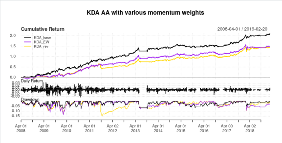
So, one mea culpa: after comparing AllocateSmartly, my initial code (which I’ve since edited, most likely owing to getting some logic mixed up when I added functionality to lag the day of month to trade) had some sort of bug in it which gave a slightly better than expected 2015 return. Nevertheless, the results are very similar. What is interesting to note is that in the raging bull market that was essentially from 2010 onwards, the equal weight and reverse weight filters don’t perform too badly, though the reverse weight filter has a massive drawdown in 2011, but in terms of capitalizing in awful markets, the original filter as designed by Keller and TrendXplorer works best, both in terms of making money during the recession, and does better near the market bottom in 2009.

Now that that’s out of the way, the more interesting question is how does the strategy work when not trading at the end of the month? Long story short, the best time to trade it is in the last week of the month. Once the new month rolls around, hands off. If you’re talking about tranching this strategy, then you have about a week’s time to get your positions in, so I’m not sure the actual dollar volume this strategy can manage, as it’s dependent on the month-end effect (I know that one of my former managers–a brilliant man, by all accounts–said that this phenomena no longer existed, but I feel these empirical results refute that assertion in this particular instance). Here are these results:

lagCompare <- list()
for(i in 1:21) {
  offRets <- KDA(rets, leverageFactor = 1, offset = i)
  tmp <- offRets[[2]]
  colnames(tmp) <- paste0("Lag", i)
  lagCompare[[i]] <- tmp
}
lagCompare <- do.call(cbind, lagCompare)
lagCompare <- na.omit(cbind(KDA_100[[2]], lagCompare))
colnames(lagCompare)[1] <- "Base"

charts.PerformanceSummary(lagCompare, colorset=c("orange", rep("gray", 21)))
stratStats(lagCompare)

With the results:

> stratStats(lagCompare)
                                Base      Lag1      Lag2      Lag3      Lag4      Lag5      Lag6      Lag7      Lag8
Annualized Return         0.11230000 0.0584000 0.0524000 0.0589000 0.0319000 0.0319000 0.0698000 0.0790000 0.0912000
Annualized Std Dev        0.09100000 0.0919000 0.0926000 0.0945000 0.0975000 0.0957000 0.0943000 0.0934000 0.0923000
Annualized Sharpe (Rf=0%) 1.23480000 0.6357000 0.5654000 0.6229000 0.3270000 0.3328000 0.7405000 0.8460000 0.9879000
Worst Drawdown            0.07920363 0.1055243 0.1269207 0.1292193 0.1303246 0.1546962 0.1290020 0.1495558 0.1227749
Calmar Ratio              1.41786439 0.5534272 0.4128561 0.4558141 0.2447734 0.2062107 0.5410771 0.5282311 0.7428230
Ulcer Performance Index   4.03566328 1.4648618 1.1219982 1.2100649 0.4984094 0.5012318 1.3445786 1.4418132 2.3277271
                               Lag9     Lag10     Lag11     Lag12     Lag13     Lag14     Lag15     Lag16     Lag17
Annualized Return         0.0854000 0.0863000 0.0785000 0.0732000 0.0690000 0.0862000 0.0999000 0.0967000 0.1006000
Annualized Std Dev        0.0906000 0.0906000 0.0900000 0.0913000 0.0906000 0.0909000 0.0923000 0.0947000 0.0949000
Annualized Sharpe (Rf=0%) 0.9426000 0.9524000 0.8722000 0.8023000 0.7617000 0.9492000 1.0825000 1.0209000 1.0600000
Worst Drawdown            0.1278059 0.1189949 0.1197596 0.1112761 0.1294588 0.1498408 0.1224511 0.1290538 0.1274083
Calmar Ratio              0.6682006 0.7252411 0.6554796 0.6578231 0.5329880 0.5752771 0.8158357 0.7493000 0.7895878
Ulcer Performance Index   2.3120919 2.6415855 2.4441605 1.9248615 1.8096134 2.2378207 2.8753265 2.9092448 3.0703542
                             Lag18     Lag19     Lag20     Lag21
Annualized Return         0.097100 0.0921000 0.1047000 0.1019000
Annualized Std Dev        0.092900 0.0903000 0.0958000 0.0921000
Annualized Sharpe (Rf=0%) 1.044900 1.0205000 1.0936000 1.1064000
Worst Drawdown            0.100604 0.1032067 0.1161583 0.1517104
Calmar Ratio              0.965170 0.8923835 0.9013561 0.6716747
Ulcer Performance Index   3.263040 2.7159601 3.0758230 3.0414002

Essentially, the trade at the very end of the month is the only one with a Calmar ratio above 1, though the Calmar ratio from lag15 to lag 21 is about .8 or higher, with a Sharpe ratio of 1 or higher. So, there’s definitely a window of when to trade, and when not to–namely, the lag 1 through 5 variations have the worst performances by no small margin. Therefore, I strongly suspect that the 1-3-6-12 filter was designed around the idea of the end-of-month effect, or at least, not stress-tested for different trading days within the month (and given that longer-dated data is only monthly, this is understandable).

Nevertheless, I hope this does answer some people’s questions from the quant finance universe. I know that Corey Hoffstein of Think Newfound (and wow that blog is good from the perspective of properties of trend-following) loves diversifying across every bit of the process, though in this case, I do think there’s something to be said about “diworsification”.

In any case, I do think there are some future research venues for further research here.

Thanks for reading.