
From area under the curve to the fundamental theorem of calculus
Want to share your content on R-bloggers? click here if you have a blog, or here if you don't.
This is a lecture post for my students in the CUNY MS Data Analytics program. In this series of lectures I discuss mathematical concepts from different perspectives. The goal is to ask questions and challenge standard ways of thinking about what are generally considered basic concepts. Consequently these lectures will not always be as rigorous as they could be.
This week let’s take a closer look at integration. People often describe integration as area under the curve. This is indeed true, yet I always found it a bit difficult to understand how you get from area under the curve to the Fundamental Theorem of Calculus. This theorem can be cast two different ways, and I’m referring to it as  dx = F(b) - F(a)")


I like starting with simple examples since it’s a lot easier to understand the behavior of something when you minimize the variables introduced. Hence, let’s start by looking at a line.
xs <- seq(-1,5, by=0.02)
f <- function(x) x - 1
plot(xs, f(xs), type='l', col='green')
abline(h=0, v=0, col='grey')

There’s nothing particularly remarkable here, so let’s change that. What happens if we add to this graph the cumulative Riemann sum of  = \sum_{k=-1}^x f(k) \Delta x")
lines(xs, cumsum(f(xs)*.02), col='blue')
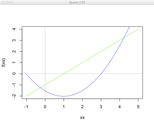
Well this looks kind of like a parabola, and obviously the limit is, but what’s the intuition around it? The simplest thing to do is to see what the cumulative sum of  \Delta x")
head(cumsum(f(xs)*.02), 20)
 [1] -0.0400 -0.0796 -0.1188 -0.1576 -0.1960 -0.2340 -0.2716 -0.3088 -0.3456
[10] -0.3820 -0.4180 -0.4536 -0.4888 -0.5236 -0.5580 -0.5920 -0.6256 -0.6588
[19] -0.6916 -0.7240
This is telling us that the area of a thin strip is rather small. It’s also telling us that since the slope is positive, a little bit less negative area is being added each time. Eventually something interesting happens as 

 = 0")

The second form of the Fundamental Theorem of Calculus is similar to our construction of the Riemann sum. It states that  dt = F(x) - F(a)")

 - F(a)) = F'(x) = f(x)")
 = 0")
")
Let’s explore the relationship of this version of the Fundamental Theorem of Calculus and the Riemann sum further. Both formulations describe a function in terms of a starting point up to some value 
")


 (1 - -1)}{2} = -2")
F <- function(x) sum(f(x) * .02)
> F(xs[xs <= 1])
[1] -2.02
Hence it seems reasonable that the integral for this special case is F(1), or  \Delta x = F(1) = -2")
> F(xs[xs <= 3])
[1] 1.665335e-16
Indeed, this value is close. We’ve successfully illustrated the relationship between area under the curve and the Fundamental Theorem of Calculus. However, this is the second version of the theorem and we started with the first. This second version relies on some constant point 
 = 0")
 dx")

lines(xs[xs >= 1], cumsum(f(xs[xs >= 1])*.02), col='brown')

This has the effect of shifting the parabola by 2, which is essentially ")
> F(xs[xs <= 3]) - F(xs[xs <= 1])
[1] 2.02
This gives us that  \Delta x = F(b) - F(a)")
 dx = F(b) - F(a)")
Exercises
- Why is F(xs[xs <= 1]) = -2.02 and not -2?
- What happens when you use an interval of 0.5 instead of 0.02?
- Draw the Riemann sum so that it’s value is consistent with the interval [1,3]
- Is it necessary for the initial area to be small for this approach to be correct?

R-bloggers.com offers daily e-mail updates about R news and tutorials about learning R and many other topics. Click here if you're looking to post or find an R/data-science job.
Want to share your content on R-bloggers? click here if you have a blog, or here if you don't.