
Ensuring R Generates the Same ANOVA F-values as SPSS
Want to share your content on R-bloggers? click here if you have a blog, or here if you don't.
When switching to R from SPSS a common concern among psychology researchers is that R gives the “correct” ANOVA F-values. By “correct” they simply mean F-values that match those generated by SPSS. Because ANOVA F-values in R do not match those in SPSS by default it often appears that R is “doing something wrong”. This is not the case. R simply has a different default configuration than SPSS.
The nature of the differences between SPSS and R becomes evident when there are an unequal number of participants across factorial ANOVA cells. There are a few simple steps that can be followed to ensure that R ANOVA values do indeed match those generated by SPSS. These steps involves using Type-III sums of squares for the ANOVA but there is more to it than that. I will detail the complete process in R here but a deeper discussion of the related statistical issues is provided in the excellent free e-book, Learning Statistics Using R by Dan Navarro
Initial R Data
> my.data <- read.csv("goggles.csv")
> my.data
   gender alcohol attractiveness
1       1       1             65
2       1       1             70
3       1       1             60
4       1       1             60
5       1       1             60
6       1       1             55
7       1       1             60
8       1       1             55
9       1       2             70
10      1       2             65
11      1       2             60
12      1       2             70
13      1       2             65
14      1       2             60
15      1       2             60
16      1       2             50
17      1       3             55
18      1       3             65
19      1       3             70
20      1       3             55
21      1       3             55
22      1       3             60
23      1       3             50
24      1       3             50
25      2       1             50
26      2       1             55
27      2       1             80
28      2       1             65
29      2       1             70
30      2       1             75
31      2       1             75
32      2       1             65
33      2       2             45
34      2       2             60
35      2       2             85
36      2       2             65
37      2       2             70
38      2       2             70
39      2       2             80
40      2       2             60
41      2       3             30
42      2       3             30
43      2       3             30
44      2       3             55
45      2       3             35
46      2       3             20
47      2       3             45
48      2       3             40
SPSS Analysis: The numbers below are the one’s we desire:
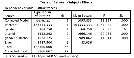
You can see the F-values for gender, alcohol, and the interaction are 2.0232, 20.065, and 11.911, respectively.
Outline of R Steps
There are three things you need to do to ensure ANOVA F-values in R match those in SPSS. I will briefly list these three steps and then provide a more details description of each.
1. Set each independent variable as a factor
2. Set the default contrast to helmert
3. Conduct analysis using Type III Sums of Squares
Step 1. Set each independent variable as a factor
By default R assumes variables are not categorical. If you have a categorical variable (as you do with ANOVA independent variables) you need to indicate to R the nature of the variables; you do this with the as.factor function. In the example below I work with a goggles data set (from Discovering Statistics Using SPSS) that investigates the effect of alcohol consumption (None,2-pints, 4-pints) and gender (male/female) or attractiveness ratings. The categorial variables have been entered into the data file numerically such that for gender 1 is Female and 2 is Male. Likewise, for alcohol 1 is None, 2 is two pints, 3 is four pints. Before running the ANOVA I need to let R know that gender and alcohol are factors and what the levels of those factors are labeled.
# Set the variables to factors
> my.data$gender <- as.factor(my.data$gender)
> my.data$alcohol <- as.factor(my.data$alcohol)

# Label the levels of each factor
> levels(my.data$gender) <- list("Female"=1,"Male"=2)
> levels(my.data$alcohol) <- list("None"=1,"2-pints"=2,"4-pints"=3)
Step 2. Set the default contrast to helmert
When an ANOVA is conducted in R it's done using the general linear model. Consequently, the contrasts need to specified in the same way as SPSS if the values are to match.
You can see the default contrasts in R with the command belowL
> options("contrasts")
$contrasts
        unordered           ordered
"contr.treatment"      "contr.poly"
We need to change the default contrast for unordered factors from "cont.treatment" to "contr.helmert". We do this with the command below:
> options(contrasts = c("contr.helmert", "contr.poly"))
You can verify that the contrast has changed by using the options command again:
> options("contrasts")
$contrasts
[1] "contr.helmert" "contr.poly"
Step 3. Conduct Analysis Using Type III Sums of Squares
Conduct your analysis:
> crf.lm <- lm(attractiveness~gender*alcohol,data=my.data)
Now you want traditional ANOVA statistics using using Type III Sums of Squares. These can be provided by the car package (car: Companion to Applied Regression). The first time (and only the first time) you use the car package you need to install it. The package give you the "Anova" function; note the capitalization in this function name is critical.
> install.packages("car",dependencies = TRUE)
Once the package is installed you only need the code below:
> crf.lm <- lm(attractiveness~gender*alcohol,data=my.data)
> library(car)
> Anova(crf.lm,type=3)
Anova Table (Type III tests)

Response: attractiveness
               Sum Sq Df   F value    Pr(>F)
(Intercept)    163333  1 1967.0251 < 2.2e-16 ***
gender            169  1    2.0323    0.1614
alcohol          3332  2   20.0654 7.649e-07 ***
gender:alcohol   1978  2   11.9113 7.987e-05 ***
Residuals        3488 42
---
Signif. codes:  0 ‘***’ 0.001 ‘**’ 0.01 ‘*’ 0.05 ‘.’ 0.1 ‘ ’ 1
You can see the F-values for gender, alcohol, and the interaction are 2.0232, 20.065, and 11.911, respectively. These match the SPSS values presented above.
Quick Summary
> my.data <- read.csv("goggles.csv")

> my.data$gender <- as.factor(my.data$gender)
> my.data$alcohol <- as.factor(my.data$alcohol)
> levels(my.data$gender) <- list("Female"=1,"Male"=2)
> levels(my.data$alcohol) <- list("None"=1,"2-pints"=2,"4-pints"=3)

> options(contrasts = c("contr.helmert", "contr.poly"))

> crf.lm <- lm(attractiveness~gender*alcohol,data=my.data)
> library(car)
> Anova(crf.lm,type=3)

Anova Table (Type III tests)

Response: attractiveness
               Sum Sq Df   F value    Pr(>F)
(Intercept)    163333  1 1967.0251 < 2.2e-16 ***
gender            169  1    2.0323    0.1614
alcohol          3332  2   20.0654 7.649e-07 ***
gender:alcohol   1978  2   11.9113 7.987e-05 ***
Residuals        3488 42
---
Signif. codes:  0 ‘***’ 0.001 ‘**’ 0.01 ‘*’ 0.05 ‘.’ 0.1 ‘ ’ 1
R-bloggers.com offers daily e-mail updates about R news and tutorials about learning R and many other topics. Click here if you're looking to post or find an R/data-science job.
Want to share your content on R-bloggers? click here if you have a blog, or here if you don't.