
Clustering
Want to share your content on R-bloggers? click here if you have a blog, or here if you don't.

Hello, everyone! I’ve been meaning to get a new blog post out for the
past couple of weeks. During that time I’ve been messing around with
clustering. Clustering, or cluster analysis, is a method of data mining
that groups similar observations together. Classification and clustering
are quite alike, but clustering is more concerned with exploration than
an end result.
Note: This post is far from an exhaustive look at all clustering has to
offer. Check out this guide
for more. I am reading Data Mining by Aggarwal presently, which is very informative.
data("iris")
head(iris)

##   Sepal.Length Sepal.Width Petal.Length Petal.Width Species
## 1          5.1         3.5          1.4         0.2  setosa
## 2          4.9         3.0          1.4         0.2  setosa
## 3          4.7         3.2          1.3         0.2  setosa
## 4          4.6         3.1          1.5         0.2  setosa
## 5          5.0         3.6          1.4         0.2  setosa
## 6          5.4         3.9          1.7         0.4  setosa
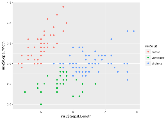
For simplicity, we’ll use the iris dataset. We’re going to try to use
the numeric data to correctly group the observations by species. There
are 50 of each species in the dataset, so ideally we would end up with
three clusters of 50.
library(ggplot2)
ggplot() +
geom_point(aes(iris$Sepal.Length, iris$Sepal.Width, col = iris$Species))

As you can see, there is already some groupings present. Let’s use
hierarcical clustering first.
iris2 <- iris[,c(1:4)]  #not going to use the `Species` column.
medians <- apply(iris2, 2, median)
mads <- apply(iris2,2,mad)
iris3 <- scale(iris2, center = medians, scale = mads)

dist <- dist(iris3)
hclust <- hclust(dist, method = 'median')  #there are several methods for hclust
cut <- cutree(hclust, 3)

table(cut)

## cut
##  1  2  3
## 49 34 67


iris <- cbind(iris, cut)
iris$cut <- factor(iris$cut)
levels(iris$cut) <- c('setosa', 'versicolor', 'virginica')
err <- iris$Species == iris$cut
table(err)

## err
## FALSE  TRUE
##    38   112


ggplot() +
geom_point(aes(iris2$Sepal.Length, iris2$Sepal.Width, col = iris$cut))
Nice groupings here, but it looks like the algorithm has some trouble
determining between versicolor and virginica. If we used this
information to classify the observations, we’d get an error rate of
about .25. Let’s try another clustering technique: DBSCAN.
library(dbscan)


db <- dbscan(iris3, eps = 1, minPts = 20)
table(db$cluster)

##
##  0  1  2
##  5 48 97


iris2 <- cbind(iris2, db$cluster)

iris2$cluster <- factor(iris2$`db$cluster`)

ggplot() +
geom_point(aes(iris2$Sepal.Length, iris2$Sepal.Width, col = iris2$cluster))
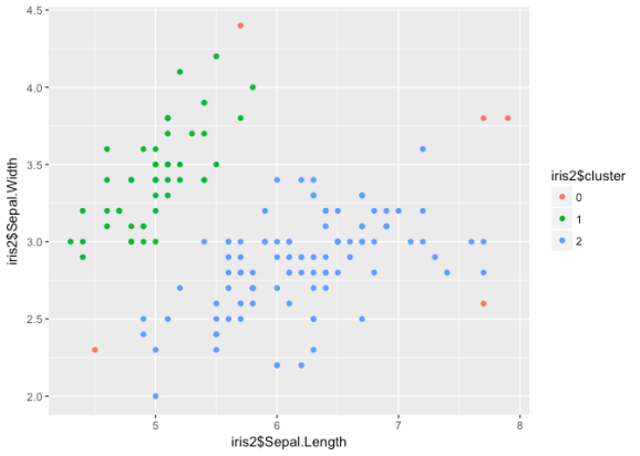
DBSCAN classifies points into three different categories: core, border,
and noise points on the basis of density. Thus, the versicolor/
virginica cluster is treated as one group. Since our data is not
structured in such a way that density is meaningful, DBSCAN is probably
not a wise choice here.
Let’s look at one last algo: the ROCK. No, not that ROCK.
library(cba)


distm <- as.matrix(dist)
rock <- rockCluster(distm, 3, theta = .02)

## Clustering:
## computing distances ...
## computing links ...
## computing clusters ...


iris$rock <- rock$cl
levels(iris$rock) <- c('setosa', 'versicolor', 'virginica')

ggplot() +
geom_point(aes(iris2$Sepal.Length, iris2$Sepal.Width, col = rock$cl))
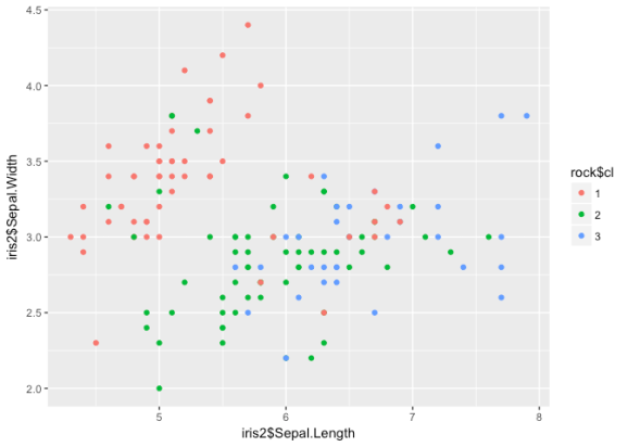
err <- (iris$Species == iris$rock)
table(err)

## err
## FALSE  TRUE
##    24   126
While it may not look like it, the ROCK does the best job at determining
clusters in this data – the error rate dropped to 16%. Typically this
method is reserved for categorical data, but since we used dist it
shouldn't cause any problems.
I have been working on a project using some of these (and similar) data
mining procedures to explore spatial data and search for distinct
groups. While clustering the iris data may not be all that meaningful,
I think it is illustrative of the power of clustering. I have yet to try
higher-dimension clustering techniques, which might be even better at
determining Species.
Have any comments? Questions? Suggestions for future posts? I am always
happy to hear from readers; please contact me!
Happy clustering,
Kiefer

R-bloggers.com offers daily e-mail updates about R news and tutorials about learning R and many other topics. Click here if you're looking to post or find an R/data-science job.
Want to share your content on R-bloggers? click here if you have a blog, or here if you don't.