
Basic assumptions to be taken care of when building a predictive model
Want to share your content on R-bloggers? click here if you have a blog, or here if you don't.
Before starting to build on a predictive model in R, the following assumptions should be taken care off;
Assumption 1: The parameters of the linear regression model must be numeric and linear in nature.
If the parameters are non-numeric like categorical then use one-hot encoding (python) or dummy encoding (R) to convert them to numeric.
Assumption 2: The mean of the residuals is Zero.
Check the mean of the residuals. If it zero (or very close), then this assumption is held true for that model. This is default unless you explicitly make amends, such as setting the intercept term to zero. Example-1 in R,
> set.seed(2)
> mod <- lm(dist ~ speed, data=cars)
> mean(mod$residuals)
[1] 8.65974e-17
Since the mean of residuals is approximately zero, this assumption holds true for this model.
Assumption 3: Homoscedasticity of residuals or equal variance:
This assumption means that the variance around the regression line is the same for all values of the predictor variable (X).
How to check?
Once the regression model is built, set
>par(mfrow=c(2, 2))
, then, plot the model using
> plot(lm.mod)
This produces four plots. The top-left and bottom-left plots shows how the residuals vary as the fitted values increase. First, I show an example where heteroscedasticity is present. To show this, I use the mtcars dataset from the base R dataset package.
> set.seed(2) # for example reproducibility
> par(mfrow=c(2,2)) # set 2 rows and 2 column plot layout
> mod_1 <- lm(mpg ~ disp, data=mtcars) # linear model
> plot(mod_1)

Figure 1: An example of heteroscedasticity in mtcars dataset
From the first plot (top-left), as the fitted values along x increase, the residuals decrease and then increase. This pattern is indicated by the red line, which should be approximately flat if the disturbances are homoscedastic. The plot on the bottom left also checks and confirms this, and is more convenient as the disturbance term in Y axis is standardized. In this case, there is a definite pattern noticed. So, there is heteroscedasticity. Lets check this on a different model. Now, I will use the cars dataset from the base r dataset package in R.
> set.seed(2) # for example reproducibility
> par(mfrow=c(2,2)) # set 2 rows and 2 column plot layout
> mod <- lm(dist ~ speed, data=cars)
> plot(mod)

Figure 2: An example of homoscedasticity in cars dataset
As seen from the first plot (top-left) the points appear random and the line looks pretty flat, with no increasing or decreasing trend. So, the condition of homoscedasticity can be accepted.
Assumption 4: No autocorrelation of residuals
Autocorrelation is specially applicable for time series data. It is the correlation of a time series with lags of itself. When the residuals are autocorrelated, it means that the current value is dependent of the previous (historic) values and that there is a definite unexplained pattern in the Y variable that shows up in the disturbances.
So how do I check for autocorrelation?
There are several methods for it like the runs test for randomness (R: lawstat::runs.test()), durbin-watson test (R: lmtest::dwtest()), acf plot from the ggplot2 library. I will use the acf plot().
# Method : Visualise with acf plot from the base R package
> ?acf # check the help page the acf function
> data(cars) # using the cars dataset from base R
> acf(cars)  # highly autocorrelated, see figure 3.
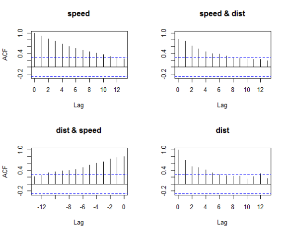
Figure 3: Detecting Auto-Correlation in Predictors
The X axis corresponds to the lags of the residual, increasing in steps of 1. The very first line (to the left) shows the correlation of residual with itself (Lag0), therefore, it will always be equal to 1.
If the residuals were not autocorrelated, the correlation (Y-axis) from the immediate next line onwards will drop to a near zero value below the dashed blue line (significance level). Clearly, this is not the case here. So we can conclude that the residuals are autocorrelated.
Remedial action to resolve Heteroscedasticity
Add a variable named resid1 (can be any name for the variable) of residual as an X variable to the original model. This can be conveniently done using the slide function in DataCombine package. If, even after adding lag1 as an X variable, does not satisfy the assumption of autocorrelation of residuals, you might want to try adding lag2, or be creative in making meaningful derived explanatory variables or interaction terms. This is more like art than an algorithm. For more details, see here
> library(DataCombine)
> set.seed(2) # for example reproducibility
> lmMod <- lm(dist ~ speed, data=cars)
> cars_data <- data.frame(cars, resid_mod1=lmMod$residuals)
> cars_data_1 <- slide(cars_data, Var="resid_mod1", NewVar = "lag1", slideBy = -1)
> cars_data_2 <- na.omit(cars_data_1)
> lmMod2 <- lm(dist ~ speed + lag1, data=cars_data_2)
> acf(lmMod2$residuals)

Figure 4: Homoscedasticity of residuals or equal variance
Assumption 5: The residuals and the X variables must be uncorrelated
How to check correlation among predictors, use the cor.test function
> set.seed(2)
> mod.lm <- lm(dist ~ speed, data=cars)
> cor.test(cars$speed, mod.lm$residuals)  # do correlation test

Pearson's product-moment correlation
data: cars$speed and mod.lm$residuals
 t = 5.583e-16, df = 48, p-value = 1
 alternative hypothesis: true correlation is not equal to 0
 95 percent confidence interval:
 -0.2783477 0.2783477
 sample estimates:
 cor
 8.058406e-17
Since p value is greater than zero, it is high, so the null hypothesis that the true correlation is Zero cannot be rejected. So the assumption holds true for this model.
Assumption 6: The number of observations must be greater than the number of predictors or X variables
This can be observed by looking at the data
Assumption 7: The variability in predictors or X values is positive
What this infers to is that the variance in the predictors should not all be the same (or even nearly the same).
How to check this in R?
var(cars$dist)
[1] 664.0608
The variance in the X variable above is much larger than 0. So, this assumption is satisfied.
Assumption 8: No perfect multicollinearity between the predictors
What this means is that there should not be a perfect linear relationship between the predictors or the explanatory variables.
How to check for multicollinearity?
Use Variance Inflation Factor (VIF). VIF is a metric computed for every X variable that goes into a linear model. If the VIF of a variable is high, it means the information in that variable is already explained by other X variables present in the given model, which means, more redundant is that variable. according to some references, if the VIF is too large(more than 5 or 10), we consider that the multicollinearity is existent. So, lower the VIF (<2) the better. VIF for a X var is calculated as:
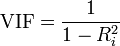
Figure 5: Variance Inflation Factor
where, Rsq is the Rsq term for the model with given X as response against all other Xs that went into the model as predictors.
Practically, if two of the X′s have high correlation, they will likely have high VIFs. Generally, VIF for an X variable should be less than 4 in order to be accepted as not causing multi-collinearity. The cutoff is kept as low as 2, if you want to be strict about your X variables.
> mod1 <- lm(mpg ~ ., data=mtcars)
> library(car) # load the car package which has the vif()
> vif(mod1)

      cyl      disp        hp      drat        wt      qsec        vs        am      gear      carb
15.373833 21.620241  9.832037  3.374620 15.164887  7.527958  4.965873  4.648487  5.357452  7.908747
From here, we can see that the VIF for data mtcars is high for all X’s variables or predictors indicating high multicollinearity.
How to remedy the issue of multicollinearity
In order to solve this problem, there are 2 main approaches. Firstly, we can use robust regression analysis instead of OLS(ordinary least squares), such as ridge regression, lasso regression and principal component regression. On the other hand, statistical learning regression is also a good method, like regression tree, bagging regression, random forest regression, neural network and SVR(support vector regression). In R language, the function lm.ridge() in package MASS could implement ridge regression(linear model). The sample codes and output as follows
library(corrplot)
corrplot(cor(mtcars[, -1]))

Correlation Plot
Assumption 9: The normality of the residuals
The residuals should be normally distributed. This can be visually checked by using the qqnorm() plot.
> par(mfrow=c(2,2))
> mod <- lm(dist ~ speed, data=cars)
> plot(mod)

Figure 6: The qqnorm plot to depict the residuals
The qqnorm() plot in top-right evaluates this assumption. If points lie exactly on the line, it is perfectly normal distribution. However, some deviation is to be expected, particularly near the ends (note the upper right), but the deviations should be small, even lesser that they are here.
Check the aforementioned assumptions automatically
The
gvlma()
from the gvlma package offers to check for the important assumptions on a given linear model.
> install.packages("gvlma")
> library(gvlma)
> par(mfrow=c(2,2))  # draw 4 plots in same window
> mod <- lm(dist ~ speed, data=cars)

Call:
lm(formula = dist ~ speed, data = cars)

Coefficients:
(Intercept)        speed
    -17.579        3.932

ASSESSMENT OF THE LINEAR MODEL ASSUMPTIONS
USING THE GLOBAL TEST ON 4 DEGREES-OF-FREEDOM:
Level of Significance =  0.05

Call:
 gvlma::gvlma(x = mod)

                    Value  p-value                   Decision
Global Stat        15.801 0.003298 Assumptions NOT satisfied!
Skewness            6.528 0.010621 Assumptions NOT satisfied!
Kurtosis            1.661 0.197449    Assumptions acceptable.
Link Function       2.329 0.126998    Assumptions acceptable.
Heteroscedasticity  5.283 0.021530 Assumptions NOT satisfied!

> plot(mod)
Three of the assumptions are not satisfied. This is probably because we have only 50 data points in the data and having even 2 or 3 outliers can impact the quality of the model. So the immediate approach to address this is to remove those outliers and re-build the model. Take a look at the diagnostic plot below.
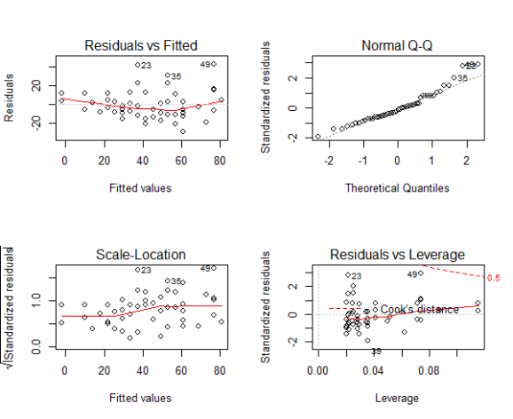
Figure 7: The diagnostic plot
As we can see in the above plot (figure 7), the data points: 23, 35 and 49 are marked as outliers. Lets remove them from the data and re-build the model.
> mod <- lm(dist ~ speed, data=cars[-c(23, 35, 49), ])
> gvlma::gvlma(mod)

Call:
lm(formula = dist ~ speed, data = cars[-c(23, 35, 49), ])

Coefficients:
(Intercept)        speed
    -15.137        3.608


ASSESSMENT OF THE LINEAR MODEL ASSUMPTIONS
USING THE GLOBAL TEST ON 4 DEGREES-OF-FREEDOM:
Level of Significance =  0.05

Call:
 gvlma::gvlma(x = mod)

                    Value p-value                Decision
Global Stat        7.5910 0.10776 Assumptions acceptable.
Skewness           0.8129 0.36725 Assumptions acceptable.
Kurtosis           0.2210 0.63831 Assumptions acceptable.
Link Function      3.2239 0.07257 Assumptions acceptable.
Heteroscedasticity 3.3332 0.06789 Assumptions acceptable.
Post removing the outliers we can see from the results that all our assumptions have been met in the new model.
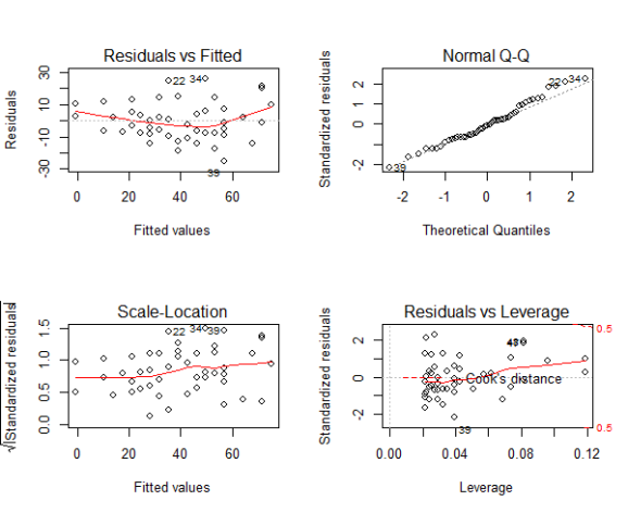
Figure 8: Normalised variables plot
Note: For a good regression model, the red smoothed line should stay close to the mid-line and no point should have a large cook’s distance (i.e. should not have too much influence on the model.). On plotting the new model, the changes look minor, it is more closer to conforming with the assumptions.
End thoughts
Given a dataset, its very important to first ensure that it fulfills the aforementioned assumptions before you begin with any sort or inferential or predictive modelling. Moreover, by taking care of these assumptions you are ensuring a robust model that will survive and yield high predictive values.
Filed under: Data Analysis & Statistics, pre-processing, R Tagged: linear regression, pre-processing, R


R-bloggers.com offers daily e-mail updates about R news and tutorials about learning R and many other topics. Click here if you're looking to post or find an R/data-science job.
Want to share your content on R-bloggers? click here if you have a blog, or here if you don't.