
24 Days of R: Day 19
Want to share your content on R-bloggers? click here if you have a blog, or here if you don't.
Carrying on with the multi-level model, I'm going to look at the paid and incurred workers comp losses for a large number of insurance companies. This is a similar exercise to what I did last night, but I'm now working with real, rather than simulated data and the stochastic process is assumed to be different.
First, I'll fetch some data from the CAS. I'm only going to look at paid and incurred losses in the first development period. I'd love to chat about the relative merits of multiplicative vs. additive chain ladder, but some other time. Tonight, I'll use data that's effectively meaningless in a chain ladder context.
URL = "http://www.casact.org/research/reserve_data/wkcomp_pos.csv"
df = read.csv(URL, stringsAsFactors = FALSE)
df = df[, c(2:7, 11)]
colnames(df) = c("GroupName", "LossPeriod", "DevelopmentYear", "DevelopmentLag",
"CumulativeIncurred", "CumulativePaid", "NetEP")
df = df[df$DevelopmentLag == 1, ]
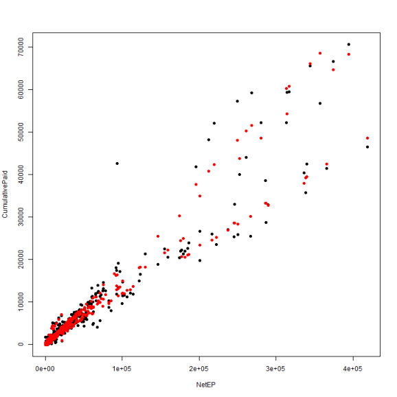
plot(CumulativeIncurred ~ NetEP, data = df, pch = 19, ylab = "Loss", xlab = "Net earned premium")
points(df$NetEP, df$CumulativePaid, pch = 19, col = "red")
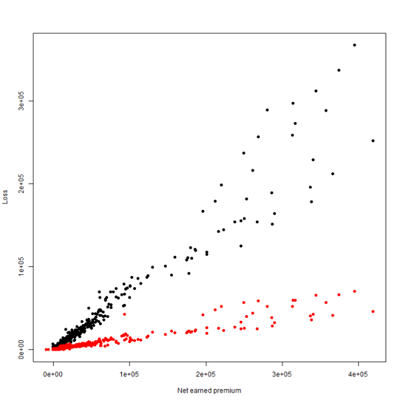
The first couple things I notice is that both sets have some inherent volatility and when plotting against earned premium, we'll probably see some heteroskedasticity in the fit. However, a linear fit looks to be a fairly safe call for the lower premium observations. There are also some erroneous values- premium shouldn't be negative. I'll eliminate the bogus premium observations and also look the losses on a log scale so that the points on the left are easier to observe.
df = df[df$NetEP > 0, ]

plot(log(CumulativeIncurred) ~ NetEP, data = df, pch = 19, ylab = "Loss", xlab = "Net earned premium")
points(df$NetEP, log(df$CumulativePaid), pch = 19, col = "red")
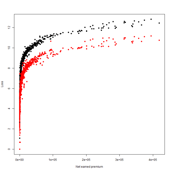
The log doesn't help loads. Really, all that it does is suggest that there are two pretty good fit lines. As with the data from yesterday, I'll perform one fit using the grouped data and another where each company is fit individually.
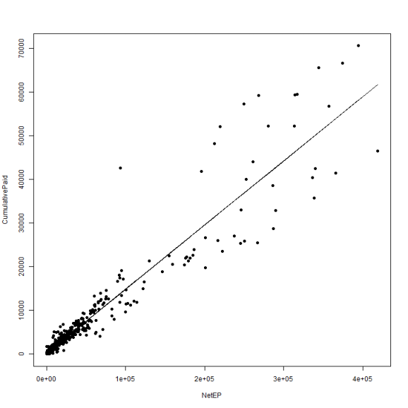
fitPool = lm(CumulativePaid ~ 1 + NetEP, data = df)
summary(fitPool)

##
## Call:
## lm(formula = CumulativePaid ~ 1 + NetEP, data = df)
##
## Residuals:
##    Min     1Q Median     3Q    Max
## -15210   -193   -131    134  28766
##
## Coefficients:
##             Estimate Std. Error t value Pr(>|t|)
## (Intercept) 1.36e+02   8.65e+01    1.58     0.12
## NetEP       1.47e-01   1.44e-03  101.80   <2e-16 ***
## ---
## Signif. codes:  0 '***' 0.001 '**' 0.01 '*' 0.05 '.' 0.1 ' ' 1
##
## Residual standard error: 2510 on 979 degrees of freedom
## Multiple R-squared:  0.914,  Adjusted R-squared:  0.914
## F-statistic: 1.04e+04 on 1 and 979 DF,  p-value: <2e-16

df$PoolPaid = predict(fitPool)
plot(CumulativePaid ~ NetEP, data = df, pch = 19)
lines(df$NetEP, df$PoolPaid)
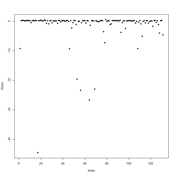
fitSplit = lm(CumulativePaid ~ 1 + NetEP:GroupName, data = df)
plot(coef(fitSplit)[abs(coef(fitSplit)) < 50], pch = 19, ylab = "Slope")
df$SplitPaid = predict(fitSplit)
plot(CumulativePaid ~ NetEP, data = df, pch = 19)
points(df$NetEP, df$SplitPaid, col = "red", pch = 19)

Lots of negative slopes and a great deal of variation when we fit each company separately. How does a blended model look?
library(lme4)
fitBlended = lmer(CumulativePaid ~ NetEP + (0 + NetEP | GroupName), data = df)
df$BlendedPaid = predict(fitBlended)

plot(CumulativePaid ~ NetEP, data = df, pch = 19)
points(df$NetEP, df$BlendedPaid, col = "red", pch = 19)
One way to measure the performance of the model is to compute the root mean squared error of prediction
rmsePool = sqrt(sum((df$PoolPaid - df$CumulativePaid)^2))
rmseSplit = sqrt(sum((df$Split - df$CumulativePaid)^2))
rmseBlended = sqrt(sum((df$BlendedPaid - df$CumulativePaid)^2))
In this case, the split model- noise and all- works best. Usual caveats apply: this works for this data set only, there ought to be cross validation, measurement against out of sample data, etc.
By the way, a really fantastic introduction to mixed effects regression may be found at AnythingButRBitrary.
Tomorrow: Meh.
sessionInfo()

## R version 3.0.2 (2013-09-25)
## Platform: x86_64-w64-mingw32/x64 (64-bit)
##
## locale:
## [1] LC_COLLATE=English_United States.1252
## [2] LC_CTYPE=English_United States.1252
## [3] LC_MONETARY=English_United States.1252
## [4] LC_NUMERIC=C
## [5] LC_TIME=English_United States.1252
##
## attached base packages:
## [1] stats     graphics  grDevices utils     datasets  methods   base
##
## other attached packages:
##  [1] knitr_1.5        RWordPress_0.2-3 lme4_1.0-5       Matrix_1.1-0
##  [5] lattice_0.20-23  plyr_1.8         lmtest_0.9-32    zoo_1.7-10
##  [9] lubridate_1.3.2  ggplot2_0.9.3.1  reshape2_1.2.2
##
## loaded via a namespace (and not attached):
##  [1] colorspace_1.2-4   dichromat_2.0-0    digest_0.6.4
##  [4] evaluate_0.5.1     formatR_0.10       grid_3.0.2
##  [7] gtable_0.1.2       labeling_0.2       MASS_7.3-29
## [10] memoise_0.1        minqa_1.2.1        munsell_0.4.2
## [13] nlme_3.1-111       proto_0.3-10       RColorBrewer_1.0-5
## [16] RCurl_1.95-4.1     scales_0.2.3       splines_3.0.2
## [19] stringr_0.6.2      tools_3.0.2        XML_3.98-1.1
## [22] XMLRPC_0.3-0

R-bloggers.com offers daily e-mail updates about R news and tutorials about learning R and many other topics. Click here if you're looking to post or find an R/data-science job.
Want to share your content on R-bloggers? click here if you have a blog, or here if you don't.