I will look at estimates for both R_t and R_u. The estimates for R_t are needed in any case in order to produce the estimates for R_u. I will also look at the 21-day averaged estimates for R_u that were used by Kissler, et al.

Interpolating to produce daily incidence proxies

The formulas for R_t and R_u above require daily data on new infections, b(t). But the incidence proxies that are used by Kissler, et al., which I discussed in Part 2 of this series, are aggregated over weeks.

As discussed below, a suitable generative interval distribution for these coronaviruses puts significant probability on intervals of only a few days, so switching to a discrete-time representation in terms of weeks would substantially distort the results. Instead, Kissler, et al. interpolate the weekly incidence proxies to daily values. This is done by a procedure described in the supplementary material of a paper by te Beest, et al., as follows:

1. The weekly incidence proxy for a virus is used to produce a weekly proxy for cumulative incidence.
2. An interpolating spline is fit to the weekly cumulative incidence proxy (passing exactly through the data points).
3. The values of this spline are evaluated at daily intervals, producing a daily proxy for cumulative incidence.
4. Differences of successive values of this daily cumulative incidence proxy are taken, producing a proxy for daily incidence.

And advantage of this procedure emphasized by te Beest, et al. is that the total incidence in the daily series exactly matches the total incidence in the original weekly series. When the weekly incidence series is a noisy and likely biased measure of true incidence, this does not seem to be a compelling justification.

A disadvantage of this procedure is that it can produce negative values for daily incidence. When applied to the proxies used by Kissler, et al. (what I call proxyW in Part 2), there are 6 negative values for NL63, 30 for 229E, none for OC43, and 89 for HKU1. Kissler, et al. replace these negative values with 10^-7.

I’ve looked at how the other proxies I discuss in Part 2 fare in this regard. Fixing the holiday anomalies only slight improves matters — proxyWX, for example, which has a fudge for holidays, has only one fewer negative daily values than proxyW. Adjusting for outliers and zeros in the fraction of positive tests for each coronavirus has a bigger effect — proxyWXo, for example, has 2 negative values for NL63, 9 for 229E, none for OC43, and 38 for HKU1.

Negative daily incidence values are completely eliminated when the fractions of positive coronavirus tests that are for each virus are smoothed, as described in Part 2 (proxyWs and proxyAXn, for example, have no negative values).

Negative values can also be reduced by applying a filter to smooth the daily values after step 4 above. I use a filter with impulse response (0.04,0.07,0.10,0.17,0.24,0.17,0.10,0.07,0.04). After this filtering, proxyWXo has only 14 negative values (all for HKU1).

Note that it may be desirable to smooth at either or both of these stages beyond the amount needed to just eliminate negative daily incidence values, since values only slightly greater than zero may also be undesirable. I’ll show below what the effects of this smoothing are on estimates for R.

The generative interval distribution used

The formulas from above — R_t = b(t) / ∑_a b(t-a)g(a) and R_u = ∑_t g(t-u)R_t — involve the generative interval distribution, g(a). Estimation of g requires information on timing and source of infections that is not captured by the incidence proxy. Due to an absence of studies on the generative interval distribution for the common cold coronaviruses, Kissler, et al. used an estimate for the serial interval distribution of SARS (a betacoronavirus related to SARS-CoV-2).

The serial interval distribution is the distribution of the time from the onset of symptoms of one infected person to the onset of symptoms for another person whom they infect. If the incubation period (time from infection to developing symptoms) were the same for all people, the serial interval distribution would be the same as the generative interval distribution — the delay from infection to symptoms for the first person would be cancelled by the same delay from infection to symptoms for the person they infect. Since the incubation period is actually at least somewhat variable, the serial interval distribution will typically have a higher variance than the generative interval distribution, although their means will be the same. (See this paper for a more detailed discussion.)

In the Kissler, et al paper, using a serial interval distribution as they do is actually more appropriate than using a generative interval distribution, since the incidence proxies are not proxies for numbers of people infected each week, but rather for the number who come to the attention of the health care system each week. If people seek medical care a fixed time after developing symptoms, the serial interval distribution would be appropriate to use. (Of course, there is actually some variation in how long people wait before seeking medical care.)

The serial interval distribution used by Kissler, et al. is derived from a Weibull distribution with shape parameter 2.35 and scale parameter 9.48 (which has mean 8.4). This is a bit funny, since Weibull distributions are continuous, but a discrete distribution is needed here. Kissler, et al. just evaluate the Weibull probability density at integer points, up to the integer where the right tail probability is less than 0.01. This procedure will not generally produce a discrete probability distribution in which the probabilities sum to one. In this case, the probabilities sum to 0.995, so the error is small (it will lead to R being overestimated by about 0.5%).

The estimated SARS serial interval distribution used is from this paper by Lipsitch, et al. Here is the Weibull fit together with the count data it is based on:

The Weibull model seems fairly reasonable, except that it perhaps gives intervals of one or two days too high a probability. There is, however, no real reason to use a distribution having a simple parametric form like the Weibull — a better match with reality would probably result from just estimating these 20 probabilities, while incorporating some sort of smoothness preference, as well as whatever other biological knowledge might be available to supplement the data.

Estimates found using various proxies for incidence

Using the daily incidence values interpolated from weekly numbers, b(t), and the chosen generative/serial interval distribution, g(a), Kissler, et al. obtain daily estimates for R_t and R_u using the formulas above. Weekly estimates for these R values can then be obtained by taking the geometric average of the values for the 7 days within each week. Kissler, et al. obtain smoothed weekly values by averaging over the 21 days in each week and its preceding and following weeks.

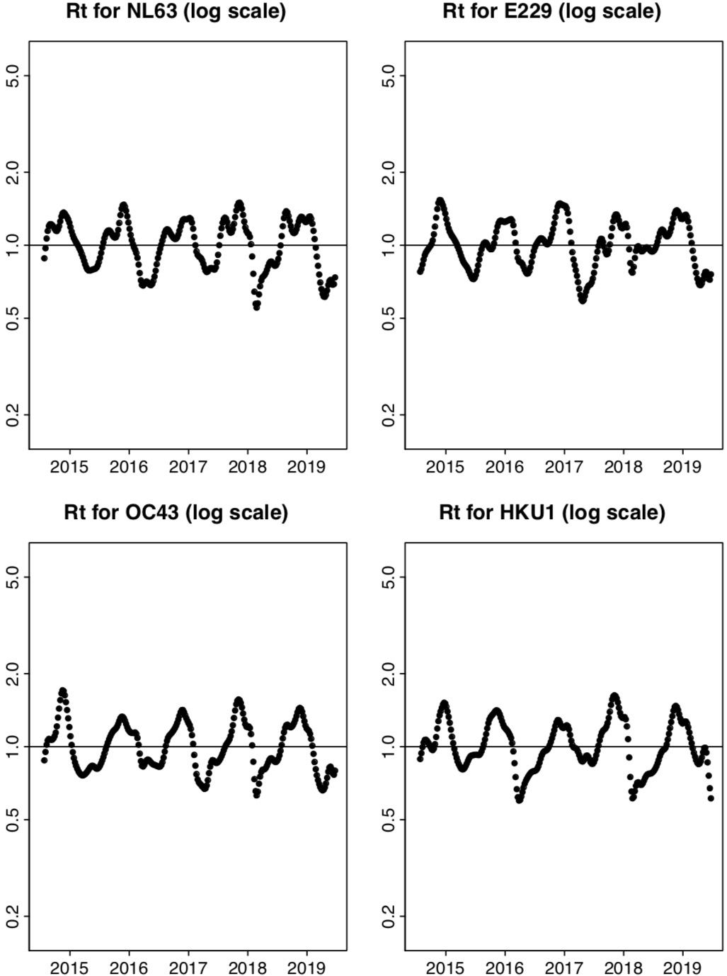
Here are the smoothed weekly values for R_u found using proxyW, the proxy used by Kissler, et al. (click for larger version):

One can see some variability that looks like it must be noise, especially for HKU1. Here are the values for R_u without smoothing:

The red points represent values that are beyond the scale of the plot.

There’s quite a bit more noise in the plots of R_u without smoothing, which may be why Kissler, et al. thought it would be beneficial to model the smoothed estimates of R_u. The benefit is illusory, however. As I’ll discuss more in the next part of this series, Kissler, et al. use a simple least-squares linear regression model for the log of these estimates. The geometric average used for smoothing R_u corresponds to a simple average for the logs. The reduction in noise from this averaging will help to no greater extent than the least-squares fitting procedure copes with noise in any case. But the averaging might obscure some relationships, and will introduce correlations in the residuals from the regression that complicate assessments of uncertainty.

I argued above that it would be better to model R_t than R_u. Here are the estimates for R_t found using proxyW:

There’s a huge amount of noise here. I’ll show in the next post that fitting a model using these R_t estimates produces ridiculous results. So if Kissler, et al. ever considered modelling R_t, one can see why they might have abandoned the idea.

Recall from above that R_u is estimated from the equation R_u = ∑_t g(t-u)R_t. So the R_u estimates are weighted averages of R_t estimates. Crucially, the averaging is done on R_t itself, not its logarithm, and so has a much different effect than the averaging that is done to smooth the R_u values. In particular, some values for R_t could be zero or close to zero, without this producing any R_u values that are close to zero. This is why the estimates for R_u don’t look as bad as those for R_t.

The real problem, however, is that proxyW, used by Kissler, et al., has multiple problems, as discussed in Part 2 of this series. Better R_t estimates can be found using proxyWXss, which fixes the problem with holidays, fixes outliers in the coronavirus data, replaces zeros in the coronavirus data with suitable non-zero values, and smooths the percentages of positive tests for each virus amongst all positive coronavirus tests. Here are these R_t estimates:

These seem much more usable. Of course, the estimates for R_u and their smoothed versions also have less noise when proxyWXss is used rather than proxyW.

Using some of the other proxies discussed in Part 2 gives estimates with even less noise. Here are the R_t estimates found using proxyDn, with filtering applied to the daily proxies:

After writing Part 2, it occurred to me that by replacing the ILI proxy by its spline fit, one can create a proxy, which I call proxyEn, that is entirely based on spline fits. Such a proxy can directly produce daily values, without any need for the interpolation procedure above. Here are the R_t estimates produced using this proxy:

Future posts

In my next post, I’ll discuss the regression model that Kissler, et al. fit to their estimates of R, especially for the two betacoronaviruses that are related to SARS-CoV-2. This model has terms for immunity, cross-immunity, and seasonal effects. I will discuss problems with this model, and with how the authors interpret the results from fitting it, and look at alternatives. In subsequent  posts, I’ll discuss the later parts of the paper, which model the incidence proxies in a different way using a SEIRS model, which is then extended to include SARS-CoV-2. This SEIRS model is the basis for their results that are intended to provide some policy guidance.