
An unofficial vignette for the gamsel package
Want to share your content on R-bloggers? click here if you have a blog, or here if you don't.
I’ve been working on a project/package that closely mirrors that of GAMSEL (generalized additive model selection), a method for fitting sparse generalized additive models (GAMs). In preparing my package, I realized that (i) the gamsel package which implements GAMSEL doesn’t have a vignette, and (ii) I could modify the vignette for my package minimally to create one for gamsel. So here it is!
For a markdown version of the vignette, go here. Unfortunately LaTeX doesn’t play well on Github… The Rmarkdown file is available here: you can download it and knit it on your own machine.
Introduction
This is an unofficial vignette for the gamsel package. GAMSEL (Generalized Additive Model Selection) is a method for fitting sparse generalized additive models proposed by Alexandra Chouldechova and Trevor Hastie. Here is the abstract of the paper:
We introduce GAMSEL (Generalized Additive Model Selection), a penalized likelihood approach for fitting sparse generalized additive models in high dimension. Our method interpolates between null, linear and additive models by allowing the effect of each variable to be estimated as being either zero, linear, or a low-complexity curve, as determined by the data. We present a blockwise coordinate descent procedure for efficiently optimizing the penalized likelihood objective over a dense grid of the tuning parameter, producing a regularization path of additive models. We demonstrate the performance of our method on both real and simulated data examples, and compare it with existing techniques for additive model selection.
Let there be 


For each variable 


where 
For more details on the method, see the arXiv paper. For `gamsel`’s official R documentation, see this link.
The gamsel() function
The purpose of this section is to give users a general sense of the gamsel() function, which is probably the most important function of the package. First, we load the gamsel package:
library(gamsel)
#> Loading required package: foreach
#> Loading required package: mda
#> Loading required package: class
#> Loaded mda 0.4-10
#> Loaded gamsel 1.8-1
Let’s generate some data:
set.seed(1)
n <- 100; p <- 12
x = matrix(rnorm((n) * p), ncol = p)
f4 = 2 * x[,4]^2 + 4 * x[,4] - 2
f5 = -2 * x[, 5]^2 + 2
f6 = 0.5 * x[, 6]^3
mu = rowSums(x[, 1:3]) + f4 + f5 + f6
y = mu + sqrt(var(mu) / 4) * rnorm(n)
We fit the model using the most basic call to gamsel():
fit <- gamsel(x, y)
The function gamsel() fits GAMSEL for a path of lambda values and returns a gamsel object. Typical usage is to have gamsel() specify the lambda sequence on its own. (By default, the model is fit for 50 different lambda values.) The returned gamsel object contains some useful information on the fitted model. For a given value of the 
where 

Printing the returned gamsel object tells us how many features, linear components and non-linear components were included in the model for each lambda value respectively. It also shows the fraction of null deviance explained by the model and the lambda value for that model.
fit
#>
#> Call:  gamsel(x = x, y = y)
#>
#>       NonZero Lin NonLin    %Dev  Lambda
#>  [1,]       0   0      0 0.00000 80.1300
#>  [2,]       1   1      0 0.03693 72.9400
#>  [3,]       1   1      0 0.06754 66.4000
#>  [4,]       1   1      0 0.09290 60.4400
#>  [5,]       1   1      0 0.11390 55.0200
#>  [6,]       1   1      0 0.13130 50.0900
#>  [7,]       1   1      0 0.14580 45.5900
#>  .... (redacted for conciseness)
gamsel has a tuning parameter gamma which is between 0 and 1. Smaller values of gamma penalize the linear components less than the non-linear components, resulting in more linear components for the fitted model. The default value is gamma = 0.4.
fit2 <- gamsel(x, y, gamma = 0.8)
By default, each variable is given 
degrees option, and this value can differ from variable to variable (to allow for this, pass a vector of length equal to the number of variables to the degrees option).
By default, the maximum degrees of freedom for each variable is 5. This can be modified with the dfs option, with larger values allowing more “wiggly” fits. Again, this value can differ from variable to variable.
Predictions
Predictions from this model can be obtained by using the predict method of the gamsel() function output: each column gives the predictions for a value of lambda.
# get predictions for all values of lambda
all_predictions <- predict(fit, x) dim(all_predictions) #> [1] 100  50

# get predictions for 20th model for first 5 observations
all_predictions[1:5, 20]
#> [1]  1.88361056 -4.47189543  8.05935149 -0.04271584  5.93270321
One can also specify the lambda indices for which predictions are desired:
# get predictions for 20th model for first 5 observations
predict(fit, x[1:5, ], index = 20)
#>              l20
#> [1,]  1.88361056
#> [2,] -4.47189543
#> [3,]  8.05935149
#> [4,] -0.04271584
#> [5,]  5.93270321
The predict method has a type option which allows it to return different types of information to the user. type = "terms" gives a matrix of fitted functions, with as many columns as there are variables. This can be useful for understanding the effect that each variable has on the response. Note that what is returned is a 3-dimensional array!
# effect of variables for first 10 observations and 20th model
indiv_fits <- predict(fit, x[1:10, ], index = c(20), type = "terms") dim(indiv_fits) #> [1] 10  1 12
# effect of variable 4 on these first 10 observations
plot(x[1:10, 4], indiv_fits[, , 4])

type = "nonzero" returns a list of indices of non-zero coefficients at a given lambda.
# variables selected by GAMSEL and the 10th and 50th lambda values
predict(fit, x, index = c(10, 50), type = "nonzero")
#> $l10
#> [1] 2 3 4 5 6
#>
#> $l50
#>  [1]  1  2  3  4  5  6  7  8  9 10 11 12
Plots and summaries
Let’s fit the basic gamsel model again:
fit <- gamsel(x, y)
fit is a class “gamsel” object which comes with a plot method. The plot method shows us the relationship our predicted response has with each input feature, i.e. it plots 
fit to the plot() call, the user must also pass an input matrix x: this is used to determine the coordinate limits for the plot. It is recommended that the user simply pass in the same input matrix that the GAMSEL model was fit on.
By default, plot() gives the fitted functions for the last value of the lambda key in fit, and gives plots for all the features. For high-dimensional data, this latter default is problematic as it will produce too many plots! You can pass a vector of indices to the which option to specify which features you want plots for. The code below gives plots for the first 4 features:
par(mfrow = c(1, 4))
par(mar = c(4, 2, 2, 2))
plot(fit, x, which = 1:4)

The user can specify the index of the lambda value to show using the index option:
# show fitted functions for x2, x5 and x8 at the model for the 15th lambda value
par(mfrow = c(1, 3))
plot(fit, x, index = 15, which = c(2, 5, 8))

Linear functions are colored green, non-linear functions are colored red, while zero functions are colored blue.
Class “gamsel” objects also have a summary method which allows the user to see the coefficient profiles of the linear and non-linear features. On each plot (one for linear features and one for non-linear features), the x-axis is the
par(mfrow = c(1, 2))
summary(fit)

We can include annotations to show which profile belongs to which feature by specifying label = TRUE.
par(mfrow = c(1, 2))
summary(fit, label = TRUE)

Cross-validation
We can perform 
cv.gamsel(). It does 10-fold cross-validation by default:
cvfit <- cv.gamsel(x, y)
We can change the number of folds using the nfolds option:
cvfit <- cv.gamsel(x, y, nfolds = 5)
If we want to specify which observation belongs to which fold, we can do that by specifying the foldid option, which is a vector of length 
set.seed(3)
foldid <- sample(rep(seq(10), length = n))
cvfit <- cv.gamsel(x, y, foldid = foldid)
A cv.gamsel() call returns a cv.gamsel object. We can plot this object to get the CV curve with error bars (one standard error in each direction). The left vertical dotted line represents lambda.min, the lambda value which attains minimum CV error, while the right vertical dotted line represents lambda.1se, the largest lambda value with CV error within one standard error of the minimum CV error.
plot(cvfit)
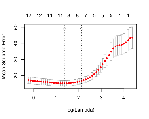
The numbers at the top represent the number of features in our original input matrix that are included in the model.
The two special lambda values, as well as their indices in the lambda path, can be extracted directly from the cv.gamsel object:
# lambda values
cvfit$lambda.min
#> [1] 3.959832
cvfit$lambda.1se
#> [1] 8.39861
# corresponding lambda indices
cvfit$index.min
#> [1] 33
cvfit$index.1se
#> [1] 25
Logistic regression with binary data
In the examples above, y was a quantitative variable (i.e. takes values along the real number line). As such, using the default family = "gaussian" for gamsel() was appropriate. In theory, the GAMSEL algorithm is very flexible and can be used when y is not a quantitative variable. In practice, gamsel() has been implemented for binary response data. The user can use gamsel() (or cv.gamsel()) to fit a model for binary data by specifying family = "binomial". All the other functions we talked about above can be used in the same way.
In this setting, the response y should be a numeric vector containing just 0s and 1s. When doing prediction, note that by default predict() gives just the value of the linear predictors, i.e.
![\begin{aligned} \log [\hat{p} / (1 - \hat{p})] = \hat{y} = \alpha_0 + \sum_{j=1}^p \alpha_j X_j + U_j \beta_j, \end{aligned}](https://s0.wp.com/latex.php?latex=%5Cbegin%7Baligned%7D+%5Clog+%5B%5Chat%7Bp%7D+%2F+%281+-+%5Chat%7Bp%7D%29%5D+%3D+%5Chat%7By%7D+%3D+%5Calpha_0+%2B+%5Csum_%7Bj%3D1%7D%5Ep+%5Calpha_j+X_j+%2B+U_j+%5Cbeta_j%2C+%5Cend%7Baligned%7D&bg=ffffff&%23038;fg=333333&%23038;s=0 "\begin{aligned} \log [\hat{p} / (1 - \hat{p})] = \hat{y} = \alpha_0 + \sum_{j=1}^p \alpha_j X_j + U_j \beta_j, \end{aligned}")
where 
type = "response" to the predict() call.
# fit binary model
bin_y <- ifelse(y > 0, 1, 0)
binfit <- gamsel(x, bin_y, family = "binomial")

# linear predictors for first 5 observations at 10th model
predict(binfit, x[1:5, ])[, 10]
#> [1]  0.1293867 -0.4531994  0.4528493 -0.2539989  0.3576436

# predicted probabilities for first 5 observations at 10th model
predict(binfit, x[1:5, ], type = "response")[, 10]
#> [1] 0.5323016 0.3886003 0.6113165 0.4368395 0.5884699
R-bloggers.com offers daily e-mail updates about R news and tutorials about learning R and many other topics. Click here if you're looking to post or find an R/data-science job.
Want to share your content on R-bloggers? click here if you have a blog, or here if you don't.