MCMCvis version 0.13.1 is now on CRAN, complete with new features for summarizing and visualizing MCMC output. See HERE and HERE for posts that cover general package features. Highlights since the last CRAN version include:

• ​MCMCsummary – Specify quantiles for equal-tailed credible intervals and return highest posterior density (HPD) intervals.
• MCMCplot – Visualize posteriors from two different models on a single caterpillar plot. Useful when comparing parameter estimates across models and for visualizing shrinkage.
• MCMCplot – Produce guide lines for caterpillar plots to more easily match parameter names to caterpillars.
• MCMCplot – Specify colors for caterpillar plots.
• All functions – Summarize and visualize model output from stanreg objects produced with the rstanarm package and brms objects produced with the brms package (in addition to output produced with the rstan, rjags, R2jags, and jagsUI packages).

Below we demonstrate how one might use some of these features using simulated data and simple models fit in JAGS.

Simulate some data

Let’s simulate data for 12 different groups using a generating process that assumes the means of these groups arise from a normal distribution with a constant mean and variance. In other words, we treat group as a ‘random effect’. We will make the groups differ in size to highlight how a random intercepts model will borrow strength compared to a model where groups are not modeled hierarchically, i.e. groups are treated as fixed effects.

# adapted from Marc Kery's WinBUGS for Ecologists (2010)
set.seed(1)
n_groups <- 12
n_obs <- rpois(n_groups, 8)
n <- sum(n_obs)
mu_group <- 20
sigma_group <- 5 
sigma <- 8
alpha <- rnorm(n_groups, mu_group, sigma_group)
epsilon <- rnorm(n, 0, sigma)
x <- rep(1:n_groups, n_obs)
X <- as.matrix(model.matrix(~as.factor(x) -1))
y <- as.numeric(X %*% as.matrix(alpha) + epsilon)
boxplot(y~x)

Fit two models to these data

First, let’s fit a simple means model to these data in JAGS where the means are not modeled hierarchically. We will use diffuse priors and let JAGS pick the initial values for simplicity’s sake.

{
sink("model1.R")
cat("
model {
# priors
for (i in 1:n_groups) { 
alpha[i] ~ dnorm(0, 0.001) 
}
sigma ~ dunif(0, 100)
tau <- 1 / sigma^2

# likelihood
for (i in 1:n) {
y[i] ~ dnorm(alpha[x[i]], tau)
}
}
", fill = TRUE)
sink()
}
data <- list(y = y, x = x, n = n, n_groups = n_groups)
params <- c("alpha", "sigma")
gvals <- c(alpha, sigma)
jm <- rjags::jags.model("model1.R", data = data, n.chains = 3, n.adapt = 5000)
jags_out1 <- rjags::coda.samples(jm, variable.names = params, n.iter = 10000

Next we fit a random intercepts model.

{
sink("model2.R")
cat("
model {
# priors
for (i in 1:n_groups) { 
alpha[i] ~ dnorm(mu_group, tau_group) 
}
mu_group ~ dnorm(0, 0.001)
sigma_group ~ dunif(0, 100)
tau_group <- 1 / sigma_group^2
sigma ~ dunif(0, 100)
tau <- 1 / sigma^2

# likelihood
for (i in 1:n) {
y[i] ~ dnorm(alpha[x[i]], tau)
}
}
", fill = TRUE)
sink()
}
data <- list(y = y, x = x, n = n, n_groups = n_groups)
params <- c("alpha", "mu_group", "sigma", "sigma_group")
gvals <- c(alpha, mu_group, sigma, sigma_group)
jm <- rjags::jags.model("model2.R", data = data, n.chains = 3, n.adapt = 5000)
jags_out2 <- rjags::coda.samples(jm, variable.names = params, n.iter = 10000)

MCMCsummary – custom equal-tailed and HPD intervals

Sample quantiles in MCMCsummary can now be specified directly using the probs argument (removing the need to define custom quantiles with the func argument). The default behavior is to provide 2.5%, 50%, and 97.5% quantiles. These probabilities can be changed by supplying a numeric vector to the probs argument. Here we ask for 90% equal-tailed credible intervals.

MCMCsummary(jags_out1, 
            params = 'alpha', 
            probs = c(0.1, 0.5, 0.9), 
            round = 2)
##            mean   sd   10%   50%   90% Rhat n.eff
## alpha[1]  23.82 3.02 19.97 23.82 27.68    1 30385
## alpha[2]  23.80 2.81 20.25 23.81 27.37    1 30000
## alpha[3]  21.83 2.63 18.49 21.83 25.18    1 29699
## alpha[4]  20.04 2.16 17.30 20.04 22.79    1 30000
## alpha[5]  29.47 3.02 25.58 29.50 33.30    1 29980
## alpha[6]  23.01 2.14 20.28 23.00 25.75    1 30305
## alpha[7]  16.20 2.06 13.60 16.20 18.84    1 30000
## alpha[8]  10.13 2.49  6.95 10.13 13.33    1 28967
## alpha[9]  26.95 2.48 23.79 26.96 30.12    1 30000
## alpha[10] 16.85 3.71 12.05 16.86 21.59    1 30262
## alpha[11] 26.10 3.03 22.24 26.11 29.96    1 30473
## alpha[12] 23.63 3.32 19.40 23.63 27.85    1 29627

Highest posterior density (HPD) intervals can now be displayed instead of equal-tailed intervals by using HPD = TRUE. This uses the HPDinterval function from the coda package to compute intervals based on the probability specified in the hpd_prob argument (this argument is different than probs argument, which is reserved for quantiles). Below we request 90% highest posterior density intervals.

MCMCsummary(jags_out1, 
            params = 'alpha', 
            HPD = TRUE, 
            hpd_prob = 0.9, 
            round = 2)
##            mean   sd 90%_HPDL 90%_HPDU Rhat n.eff
## alpha[1]  23.82 3.02    18.86    28.75    1 30385
## alpha[2]  23.80 2.81    19.20    28.45    1 30000
## alpha[3]  21.83 2.63    17.58    26.17    1 29699
## alpha[4]  20.04 2.16    16.53    23.63    1 30000
## alpha[5]  29.47 3.02    24.45    34.37    1 29980
## alpha[6]  23.01 2.14    19.66    26.63    1 30305
## alpha[7]  16.20 2.06    12.79    19.54    1 30000
## alpha[8]  10.13 2.49     6.12    14.31    1 28967
## alpha[9]  26.95 2.48    22.96    31.10    1 30000
## alpha[10] 16.85 3.71    10.79    22.98    1 30262
## alpha[11] 26.10 3.03    21.29    31.23    1 30473
## alpha[12] 23.63 3.32    18.01    28.94    1 29627

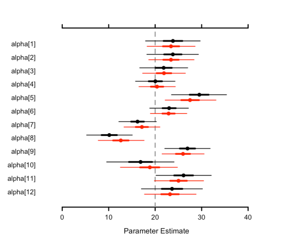
MCMCplot – multimodel visualization

Posterior estimates from two different models can also now be visualized with MCMCplot. Let’s visually compare the alpha parameter posterior samples from the fixed effect and random intercepts models to see how our choice of model affected the posterior estimates. Below we can see that the random intercepts model means (in red) are pulled towards the true (generating value) grand mean (the vertical dashed line) compared to the fixed intercepts model means (in black), as expected due to shrinkage.

MCMCplot(object = jags_out1, 
         object2 = jags_out2, 
         params = 'alpha', 
         offset = 0.2, 
         ref = mu_group)

Guide lines can also be produced (using the guide_lines argument) to help guide to eye from the parameter name to the associated caterpillar, which can be useful when trying to visualize a large number of parameters on a single plot. Colors can also be specified for each parameter (or the entire set of parameters).

MCMCplot(object = jags_out1, 
         params = 'alpha', 
         offset = 0.2, 
         guide_lines = TRUE, 
         ref = NULL, 
         col = topo.colors(12),
         sz_med = 2.5,
         sz_thick = 9,
         sz_thin = 4)

Check out the full package vignette HERE. The MCMCvis source code can be found HERE. More information on authors: Christian Che-Castaldo, Casey Youngflesh.