library(MetaLandSim)

Then we should define the characteristics of the graph-landscape. Here we are creating a landscape square with a size of 5000×5000 meters, minimum distance between patches  of 20 meters, mean area 0.8 hectares and we are using 300 -which I called dispersal ability- as a threshold to aggregate habitat patches).

Running this function  (if plotG=TRUE) will immediately plot the landscape-graph:

rl1 <- rland.graph(mapsize=5000, dist_m=20, areaM=0.8, 
        areaSD=0.2, Npatch=180,
        disp=300, plotG=TRUE)

plot_graph(rl1, species=FALSE, links=TRUE)

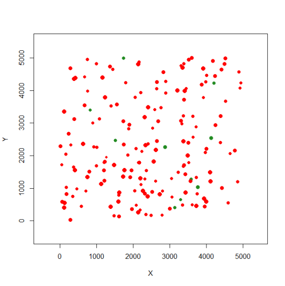
And now, we can create the first occupied landscape (here I selected 10% of the patches to be occupied, those patches in green):

sp1 <- species.graph(rl=rl1, method="number", parm=10, nsew="none", plotG=TRUE)

Again, now we don’t need to re-plot this landscape. But if that’s necessary use this:

plot_graph(sp1, species=TRUE, links=FALSE)

Starting with the previously created landscape (rl1) we now create a list containing this landscape through 100 time steps (here I did not consider any dynamics -par1=”none”-, check the manual for details, so all time steps have the same landscape):

span1 <- span.graph(rl=rl1, span=100, par1="none", par2=NULL, 
par3=NULL, par4=NULL, par5=NULL)

Now we need to define the species parameters, defining its metapopulational dynamics.

Metalandsim provides Bayesian-based functions to derive these parameters, based upon the work of Benjamin Risk in this paper (his original functions are here).

Benjamin adapted his functions to be included in this package. Later, we collaborated, and used this approach in our 2017 paper (we provided the R scripts as supplementary information, these can be downloaded from the paper’s website). This is the recommended procedure, but the package has another function (parameter.estimate). It provides some other approaches (however I don’t recommend it). It is useful sometimes, for didactic reasons, because it’s way simpler (and that is why it was not yet deprecated).

Here I’m only going to create the parameter data frame, assuming these were previously estimated.

And, finally, simulate the species occupation (considering the parameters just defined) through the time steps:

sim1 <- simulate_graph(rl=sp1,
rlist=span1,
simulate.start=FALSE,
method=NULL,
parm=NULL,
nsew="none",
succ = "none",
param_df=param1,
kern="op1",
conn="op1",
colnz="op1",
ext="op1",
beta1=NULL,
b=1,
c1=NULL,
c2=NULL,
z=NULL,
R=NULL
)

No, just to see what with the species occupation thorough time, we can plot a few of the time steps (1, 20, 40, 60, 80 and 100):

 par(mfrow=c(2,3))#we are going to 6 time steps

#First landscape
plotL.graph(rl=sp1, rlist=sim1, #time step 1
nr=1, species=TRUE, links=FALSE)

plotL.graph(rl=sp1, rlist=sim1, #time step 20
nr=20, species=TRUE, links=FALSE)

plotL.graph(rl=sp1, rlist=sim1, #time step 40
nr=40, species=TRUE, links=FALSE)

plotL.graph(rl=sp1, rlist=sim1, #time step 60
nr=60, species=TRUE, links=FALSE)

plotL.graph(rl=sp1, rlist=sim1, #time step 80
nr=80, species=TRUE, links=FALSE)

plotL.graph(rl=sp1, rlist=sim1, #time step 100
nr=100, species=TRUE, links=FALSE)

The species gradually expands from the initial occupied habitat patches (the green patches on the top left landscape-graph):

Finally, just a few reminders:

• This post was only to demonstrate the basic reasoning behind these simulations;
• The species parameters should be carefully estimated (see the Bayesian approach);
• MetaLandSim’s simulations should be repeated many times (to allow the results to stabilize). This one-run simulation was an example (for more on this, check the iterate.graph function).