This post will introduce KDA Asset Allocation. KDA — I.E. Kipnis Defensive Adaptive Asset Allocation is a combination of Wouter Keller’s and TrendXplorer’s Defensive Asset Allocation, along with ReSolve Asset Management’s Adaptive Asset Allocation. This is an asset allocation strategy with a profile unlike most tactical asset allocation strategies I’ve seen before (namely, it barely loses any money in 2015, which was generally a brutal year for tactical asset allocation strategies).

So, the idea for this strategy came from reading an excellent post from TrendXplorer on the idea of a canary universe–using a pair of assets to determine when to increase exposure to risky/aggressive assets, and when to stay in cash. Rather than gauge it on the momentum of the universe itself, the paper by Wouter Keller and TrendXplorer instead uses proxy assets VWO and BND as a proxy universe. Furthermore, in which situations say to take full exposure to risky assets, the latest iteration of DAA actually recommends leveraging exposure to risky assets, which will also be demonstrated. Furthermore, I also applied the idea of the 1-3-6-12 fast filter espoused by Wouter Keller and TrendXplorer–namely, the sum of the 12 * 1-month momentum, 4 * 3-month momentum, 2 * 6-month momentum, and the 12 month momentum (that is, month * some number = 12). This puts a large emphasis on the front month of returns, both for the risk on/off assets, and the invested assets themselves.

However, rather than adopt the universe of investments from the TrendXplorer post, I decided to instead defer to the well-thought-out universe construction from Adaptive Asset Allocation, along with their idea to use a mean variance optimization approach for actually weighting the selected assets.

So, here are the rules:

Take the investment universe–SPY, VGK, EWJ, EEM, VNQ, RWX, IEF, TLT, DBC, GLD, and compute the 1-3-6-12 momentum filter for them (that is, the sum of 12 * 1-month momentum, 4 * 3-month momentum, 2* 6-month momentum and 12 month momentum), and rank them. The selected assets are those with a momentum above zero, and that are in the top 5.

Use a basic quadratic optimization algorithm on them, feeding in equal returns (as they passed the dual momentum filter), such as the portfolio.optim function from the tseries package.

From adaptive asset allocation, the covariance matrix is computed using one-month volatility estimates, and a correlation matrix that is the weighted average of the same parameters used for the momentum filter (that is, 12 * 1-month correlation + 4 * 3-month correlation + 2 * 6-month correlation + 12-month correlation, all divided by 19).

Next, compute your exposure to risky assets by which percentage of the two canary assets–VWO and BND–have a positive 1-3-6-12 momentum. If both assets have a positive momentum, leverage the portfolio (if desired). Reapply this algorithm every month.

All of the allocation not made to risky assets goes towards IEF (which is in the pool of risky assets as well, so some months may have a large IEF allocation) if it has a positive 1-3-6-12 momentum, or just stay in cash if it does not.

The one somewhat optimistic assumption made is that the strategy observes the close on a day, and enters at the close as well. Given a holding period of a month, this should not have a massive material impact as compared to a strategy which turns over potentially every day.

Here’s the R code to do this:

# KDA asset allocation 
# KDA stands for Kipnis Defensive Adaptive (Asset Allocation).

# compute strategy statistics
stratStats <- function(rets) {
  stats <- rbind(table.AnnualizedReturns(rets), maxDrawdown(rets))
  stats[5,] <- stats[1,]/stats[4,]
  stats[6,] <- stats[1,]/UlcerIndex(rets)
  rownames(stats)[4] <- "Worst Drawdown"
  rownames(stats)[5] <- "Calmar Ratio"
  rownames(stats)[6] <- "Ulcer Performance Index"
  return(stats)
}

# required libraries
require(quantmod)
require(PerformanceAnalytics)
require(tseries)

# symbols
symbols <- c("SPY", "VGK",   "EWJ",  "EEM",  "VNQ",  "RWX",  "IEF",  "TLT",  "DBC",  "GLD", "VWO", "BND")  


# get data
rets <- list()
for(i in 1:length(symbols)) {
  
  returns <- Return.calculate(Quandl(paste0("EOD/", symbols[i]), start_date="1990-12-31", type = "xts")$Adj_Close)
  colnames(returns) <- symbols[i]
  rets[[i]] <- returns
}
rets <- na.omit(do.call(cbind, rets))


# algorithm
KDA <- function(rets, offset = 0, leverageFactor = 1.5) {
  
  # get monthly endpoints, allow for offsetting ala AllocateSmartly/Newfound Research
  ep <- endpoints(rets) + offset
  ep[ep < 1] <- 1
  ep[ep > nrow(rets)] <- nrow(rets)
  ep <- unique(ep)
  
  # initialize vector holding zeroes for assets
  emptyVec <- data.frame(t(rep(0, 10)))
  colnames(emptyVec) <- symbols[1:10]
  
  
  allWts <- list()
  # we will use the 13612F filter
  for(i in 1:(length(ep)-12)) {
    
    # 12 assets for returns -- 2 of which are our crash protection assets
    retSubset <- rets[c((ep[i]+1):ep[(i+12)]),]
    epSub <- endpoints(retSubset)
    sixMonths <- retSubset[(epSub[7]+1):epSub[13],]
    threeMonths <- retSubset[(epSub[10]+1):epSub[13],]
    oneMonth <- retSubset[(epSub[12]+1):epSub[13],]
    
    # computer 13612 fast momentum
    moms <- Return.cumulative(oneMonth) * 12 + Return.cumulative(threeMonths) * 4 + 
      Return.cumulative(sixMonths) * 2 + Return.cumulative(retSubset)
    assetMoms <- moms[,1:10] # Adaptive Asset Allocation investable universe
    cpMoms <- moms[,11:12] # VWO and BND from Defensive Asset Allocation
    
    # find qualifying assets
    highRankAssets <- rank(assetMoms) >= 6 # top 5 assets
    posReturnAssets <- assetMoms > 0 # positive momentum assets
    selectedAssets <- highRankAssets & posReturnAssets # intersection of the above
    
    # perform mean-variance/quadratic optimization
    investedAssets <- emptyVec
    if(sum(selectedAssets)==0) {
      investedAssets <- emptyVec
    } else if(sum(selectedAssets)==1) {
      investedAssets <- emptyVec + selectedAssets 
    } else {
      idx <- which(selectedAssets)
      # use 1-3-6-12 fast correlation average to match with momentum filter  
      cors <- (cor(oneMonth[,idx]) * 12 + cor(threeMonths[,idx]) * 4 + 
                 cor(sixMonths[,idx]) * 2 + cor(retSubset[,idx]))/19
      vols <- StdDev(oneMonth[,idx]) # use last month of data for volatility computation from AAA
      covs <- t(vols) %*% vols * cors
      
      # do standard min vol optimization
      minVolRets <- t(matrix(rep(1, sum(selectedAssets))))
      minVolWt <- portfolio.optim(x=minVolRets, covmat = covs)$pw
      names(minVolWt) <- colnames(covs)
      investedAssets <- emptyVec
      investedAssets[,selectedAssets] <- minVolWt
    }
    
    # crash protection -- between aggressive allocation and crash protection allocation
    pctAggressive <- mean(cpMoms > 0)
    investedAssets <- investedAssets * pctAggressive 
    
    pctCp <- 1-pctAggressive
    
    if(pctCp == 0) {}
    
    # if IEF momentum is positive, invest all crash protection allocation into it
    # otherwise stay in cash for crash allocation
    if(assetMoms["IEF"] > 0) {
      investedAssets["IEF"] <- investedAssets["IEF"] + pctCp
    }
    
    # leverage portfolio if desired in cases when both risk indicator assets have positive momentum
    if(pctAggressive == 1) {
      investedAssets = investedAssets * leverageFactor
    }
    
    # append to list of monthly allocations
    wts <- xts(investedAssets, order.by=last(index(retSubset)))
    allWts[[i]] <- wts
    
  }
  
  # put all weights together and compute cash allocation
  allWts <- do.call(rbind, allWts)
  allWts$CASH <- 1-rowSums(allWts)
  
  # add cash returns to universe of investments
  investedRets <- rets[,1:10]
  investedRets$CASH <- 0
  
  # compute portfolio returns
  out <- Return.portfolio(R = investedRets, weights = allWts)
  return(out)
}

# different leverages
KDA_100 <- KDA(rets, leverageFactor = 1)
KDA_150 <- KDA(rets, leverageFactor = 1.5)
KDA_200 <- KDA(rets, leverageFactor = 2)

# compare
compare <- na.omit(cbind(KDA_100, KDA_150, KDA_200))
colnames(compare) <- c("KDA_base", "KDA_lev_150%", "KDA_lev_200%")
charts.PerformanceSummary(compare, colorset = c('black', 'purple', 'gold'), 
                          main = "KDA AA with various offensive leverages")

And here are the equity curves and statistics:

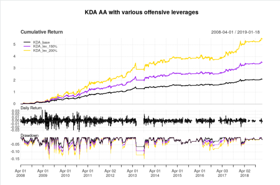
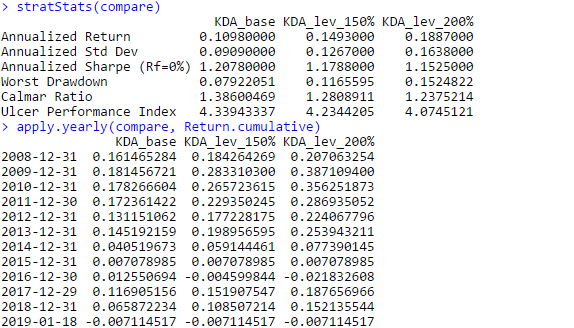
What appeals to me about this strategy, is that unlike most tactical asset allocation strategies, this strategy comes out relatively unscathed by the 2015-2016 whipsaws that hurt so many other tactical asset allocation strategies. However this strategy isn’t completely flawless, as sometimes, it decides that it’d be a great time to enter full risk-on mode and hit a drawdown, as evidenced by the drawdown curve. Nevertheless, the Calmar ratios are fairly solid for a tactical asset allocation rotation strategy, and even in a brutal 2018 that decimated all risk assets, this strategy managed to post a very noticeable *positive* return. On the downside, the leverage plan actually seems to *negatively* affect risk/reward characteristics in this strategy–that is, as leverage during aggressive allocations increases, characteristics such as the Sharpe and Calmar ratio actually *decrease*.

Overall, I think there are different aspects to unpack here–such as performances of risky assets as a function of the two canary universe assets, and a more optimal leverage plan. This was just the first attempt at combining two excellent ideas and seeing where the performance goes. I also hope that this strategy can have a longer backtest over at AllocateSmartly.

Thanks for reading.