
Problems in Estimating GARCH Parameters in R (Part 2; rugarch)
Want to share your content on R-bloggers? click here if you have a blog, or here if you don't.
Introduction
Now here is a blog post that has been sitting on the shelf far longer than it should have. Over a year ago I wrote an article about problems I was having when estimating the parameters of a GARCH(1,1) model in R. I documented the behavior of parameter estimates (with a focus on 
I was not disappointed in the feedback. You can see some mailing list feedback, and there were some comments on Reddit that were helpful, but I think the best feedback I got was through my own e-mail.
Dr. Brian G. Peterson, a member of the R finance community, sent some thought provoking e-mails. The first informed me that fGarch is no longer the go-to package for working with GARCH models. The RMetrics suite of packages (which include fGarch) was maintained by Prof. Diethelm Würtz at ETH Zürich. He was killed in a car accident in 2016.
Dr. Peterson recommended I look into two more modern packages for GARCH modelling, rugarch (for univariate GARCH models) and rmgarch (for multivariate GARCH models). I had not heard of these packages before (the reason I was aware of fGarch was because it was referred to in the time series textbook Time Series Analysis and Its Applications with R Examples by Shumway and Stoffer), so I’m very thankful for the suggestion. Since I’m interested in univariate time series for now, I only looked at rugarch. The package appears to have more features and power than fGarch, which may explain why it seems more difficult to use. However the package’s vignette is helpful and worth printing out.
Dr. Peterson also had interesting comments about my proposed applications. He argued that intraday data should be preferred to daily data and that simulated data (including simulated GARCH processes) has idiosyncracies not seen in real data. The ease of getting daily data (particularly for USD/JPY around the time of Asian financial crises, which was an intended application of a test statistic I’m studying) motivated my interest in daily data. His comments, though, may lead me to reconsider this application.1 (I might try to detect the 2010 eurozone financial crises via EUR/USD instead. I can get free intraday data from HistData.com for this.) However, if standard error estimates cannot be trusted for small sample sizes, our test statistic would still be in trouble since it involves estimating parameters even for small sample sizes.
He also warned that simulated data exhibits behaviors not seen in real data. That may be true, but simulated data is important since it can be considered a statistician’s best-case scenario. Additionally, the properties of the process that generated simulated data are known a priori, including the values of the generating parameters and whether certain hypotheses (such as whether there is a structural change in the series) are true. This allows for sanity checks of estimators and tests. This is impossible for real-world since we don’t have the a priori knowledge needed.
Prof. André Portela Santos asked that I repeat the simulations but with 


My advisor contacted another expert on GARCH models and got some feedback. Supposedly the standard error for 

So given this feedback, I will be conducting more simulation experiments. I won’t be looking at fGarch or tseries anymore; I will be working exclusively with rugarch. I will explore different optimization procedures supported by the package. I won’t be creating plots like I did in my first post; those plots were meant only to show the existence of a problem and its severity. Instead I will be looking at properties of the resulting estimators produced by different optimization procedures.
Introduction to rugarch
As mentioned above, rugarch is a package for working with GARCH models; a major use case is estimating their parameters, obviously. Here I will demonstrate how to specify a GARCH model, simulate data from the model, and estimate parameters. After this we can dive into simulation studies.
library(rugarch)


## Loading required package: parallel
##
## Attaching package: 'rugarch'
## The following object is masked from 'package:stats':
##
##     sigma
Specifying a ") model
model
To work with a GARCH model we need to specify it. The function for doing this is ugarchspec(). I think the parameters variance.model and mean.model are the most important parameters.
variance.model is a list with named entries, perhaps the two most interesting being model and garchOrder. model is a string specify which type of GARCH model is being fitted. Many major classes of GARCH models (such as EGARCH, IGARCH, etc.) are supported; for the “vanilla” GARCH model, set this to "sGARCH" (or just omit it; the standard model is the default). garchOrder is a vector for the order of the ARCH and GARCH components of the model.
mean.model allows for fitting ARMA-GARCH models, and functions like variance.model in that it accepts a list of named entries, the most interesting being armaOrder and include.mean. armaOrder is like garchOrder; it’s a vector specifying the order of the ARMA model. include.mean is a boolean that, if true, allows for the ARMA part of the model to have non-zero mean.
When simulating a process, we need to set the values of our parameters. This is done via the fixed.pars parameter, which accepts a list of named elements, the elements of the list being numeric. They need to fit the conventions the function uses for parameters; for example, if we want to set the parameters of a ")
"alpha1" and "beta1". If the plan is to simulate a model, every parameter in the model should be set this way.
There are other parameters interesting in their own right but I focus on these since the default specification is an ARMA-GARCH model with ARMA order of ")
spec1 <- ugarchspec(mean.model = list(armaOrder = c(0,0), include.mean = FALSE),
                    fixed.pars = list("omega" = 0.2, "alpha1" = 0.2,
                                      "beta1" = 0.2))
spec2 <- ugarchspec(mean.model = list(armaOrder = c(0,0), include.mean = FALSE),
                    fixed.pars = list("omega" = 0.2, "alpha1" = 0.1,
                                      "beta1" = 0.7))

show(spec1)


##
## *---------------------------------*
## *       GARCH Model Spec          *
## *---------------------------------*
##
## Conditional Variance Dynamics
## ------------------------------------
## GARCH Model		: sGARCH(1,1)
## Variance Targeting	: FALSE
##
## Conditional Mean Dynamics
## ------------------------------------
## Mean Model		: ARFIMA(0,0,0)
## Include Mean		: FALSE
## GARCH-in-Mean		: FALSE
##
## Conditional Distribution
## ------------------------------------
## Distribution	:  norm
## Includes Skew	:  FALSE
## Includes Shape	:  FALSE
## Includes Lambda	:  FALSE


show(spec2)


##
## *---------------------------------*
## *       GARCH Model Spec          *
## *---------------------------------*
##
## Conditional Variance Dynamics
## ------------------------------------
## GARCH Model		: sGARCH(1,1)
## Variance Targeting	: FALSE
##
## Conditional Mean Dynamics
## ------------------------------------
## Mean Model		: ARFIMA(0,0,0)
## Include Mean		: FALSE
## GARCH-in-Mean		: FALSE
##
## Conditional Distribution
## ------------------------------------
## Distribution	:  norm
## Includes Skew	:  FALSE
## Includes Shape	:  FALSE
## Includes Lambda	:  FALSE
Simulating a GARCH process
The function ugarchpath() simulates GARCH models specified via ugarchspec(). The function needs a specification objectect created by ugarchspec() first. The parameters n.sim and n.start specify the size of the process and the length of the burn-in period, respectively (with defaults 1000 and 0, respectively; I strongly recommend setting the burn-in period to at least 500, but I go for 1000). The function creates an object that contains not only the simulated series but also residuals and 
The rseed parameter controls the random seed the function uses for generating data. Be warned that set.seed() is effectively ignored by this function, so if you want consistent results, you will need to set this parameter.
The plot() method accompanying these objects is not completely transparent; there are a few plots it could create and when calling plot() on a uGARCHpath object in the command line users are prompted to input a number corresponding to the desired plot. This is a pain sometimes so don’t forget to pass the desired plot’s number to the which parameter to avoid the prompt; setting which = 2 will give the plot of the series proper.
old_par <- par()
par(mfrow = c(2, 2))

x_obj <- ugarchpath(spec1, n.sim = 1000, n.start = 1000, rseed = 111217)
show(x_obj)


##
## *------------------------------------*
## *     GARCH Model Path Simulation    *
## *------------------------------------*
## Model: sGARCH
## Horizon:  1000
## Simulations: 1
##                 Seed Sigma2.Mean Sigma2.Min Sigma2.Max Series.Mean
## sim1          111217       0.332      0.251      0.915    0.000165
## Mean(All)          0       0.332      0.251      0.915    0.000165
## Unconditional     NA       0.333         NA         NA    0.000000
##               Series.Min Series.Max
## sim1               -1.76       1.62
## Mean(All)          -1.76       1.62
## Unconditional         NA         NA


for (i in 1:4) {
  plot(x_obj, which = i)
}
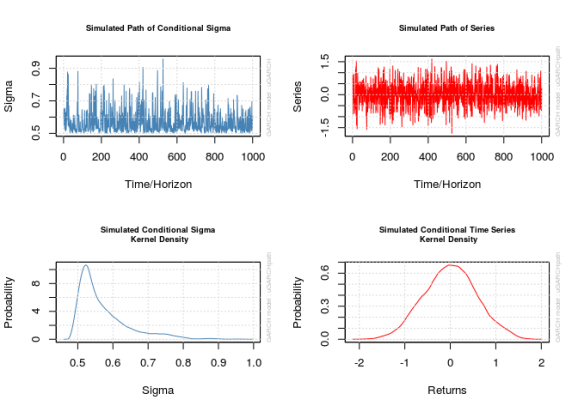
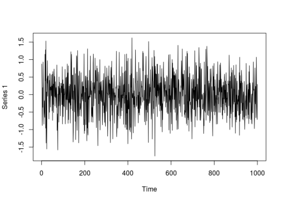
par(old_par)


## Warning in par(old_par): graphical parameter "cin" cannot be set
## Warning in par(old_par): graphical parameter "cra" cannot be set
## Warning in par(old_par): graphical parameter "csi" cannot be set
## Warning in par(old_par): graphical parameter "cxy" cannot be set
## Warning in par(old_par): graphical parameter "din" cannot be set
## Warning in par(old_par): graphical parameter "page" cannot be set


# The actual series
x1 <- x_obj@path$seriesSim
plot.ts(x1)
Fitting a model
The ugarchfit() function fits GARCH models. The function needs a specification and a dataset. The solver parameter accepts a string stating which numerical optimizer to use to find the parameter estimates. Most of the parameters of the function manage interfacing with the numerical optimizer. In particular, solver.control can be given a list of arguments to pass to the optimizer. We will be looking at this in more detail later.
The specification used for generating the simulated data won’t be appropriate for ugarchfit(), since it contains fixed values for its parameters. In my case I will need to create a second specification object.
spec <- ugarchspec(mean.model = list(armaOrder = c(0, 0), include.mean = FALSE))
fit <- ugarchfit(spec, data = x1)
show(fit)


##
## *---------------------------------*
## *          GARCH Model Fit        *
## *---------------------------------*
##
## Conditional Variance Dynamics
## -----------------------------------
## GARCH Model	: sGARCH(1,1)
## Mean Model	: ARFIMA(0,0,0)
## Distribution	: norm
##
## Optimal Parameters
## ------------------------------------
##         Estimate  Std. Error    t value Pr(>|t|)
## omega   0.000713    0.001258    0.56696  0.57074
## alpha1  0.002905    0.003714    0.78206  0.43418
## beta1   0.994744    0.000357 2786.08631  0.00000
##
## Robust Standard Errors:
##         Estimate  Std. Error    t value Pr(>|t|)
## omega   0.000713    0.001217    0.58597  0.55789
## alpha1  0.002905    0.003661    0.79330  0.42760
## beta1   0.994744    0.000137 7250.45186  0.00000
##
## LogLikelihood : -860.486
##
## Information Criteria
## ------------------------------------
##
## Akaike       1.7270
## Bayes        1.7417
## Shibata      1.7270
## Hannan-Quinn 1.7326
##
## Weighted Ljung-Box Test on Standardized Residuals
## ------------------------------------
##                         statistic p-value
## Lag[1]                      3.998 0.04555
## Lag[2*(p+q)+(p+q)-1][2]     4.507 0.05511
## Lag[4*(p+q)+(p+q)-1][5]     9.108 0.01555
## d.o.f=0
## H0 : No serial correlation
##
## Weighted Ljung-Box Test on Standardized Squared Residuals
## ------------------------------------
##                         statistic   p-value
## Lag[1]                      29.12 6.786e-08
## Lag[2*(p+q)+(p+q)-1][5]     31.03 1.621e-08
## Lag[4*(p+q)+(p+q)-1][9]     32.26 1.044e-07
## d.o.f=2
##
## Weighted ARCH LM Tests
## ------------------------------------
##             Statistic Shape Scale P-Value
## ARCH Lag[3]     1.422 0.500 2.000  0.2331
## ARCH Lag[5]     2.407 1.440 1.667  0.3882
## ARCH Lag[7]     2.627 2.315 1.543  0.5865
##
## Nyblom stability test
## ------------------------------------
## Joint Statistic:  0.9518
## Individual Statistics:
## omega  0.3296
## alpha1 0.2880
## beta1  0.3195
##
## Asymptotic Critical Values (10% 5% 1%)
## Joint Statistic:     	 0.846 1.01 1.35
## Individual Statistic:	 0.35 0.47 0.75
##
## Sign Bias Test
## ------------------------------------
##                    t-value      prob sig
## Sign Bias           0.3946 6.933e-01
## Negative Sign Bias  3.2332 1.264e-03 ***
## Positive Sign Bias  4.2142 2.734e-05 ***
## Joint Effect       28.2986 3.144e-06 ***
##
##
## Adjusted Pearson Goodness-of-Fit Test:
## ------------------------------------
##   group statistic p-value(g-1)
## 1    20     20.28       0.3779
## 2    30     26.54       0.5965
## 3    40     36.56       0.5817
## 4    50     47.10       0.5505
##
##
## Elapsed time : 2.60606


par(mfrow = c(3, 4))
for (i in 1:12) {
  plot(fit, which = i)
}


##
## please wait...calculating quantiles...
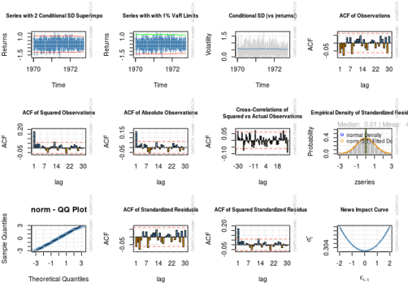
par(old_par)


## Warning in par(old_par): graphical parameter "cin" cannot be set
## Warning in par(old_par): graphical parameter "cra" cannot be set
## Warning in par(old_par): graphical parameter "csi" cannot be set
## Warning in par(old_par): graphical parameter "cxy" cannot be set
## Warning in par(old_par): graphical parameter "din" cannot be set
## Warning in par(old_par): graphical parameter "page" cannot be set
Notice the estimated parameters and standard errors? The estimates are nowhere near the “correct” numbers even for a sample size of 1000, and there is no way a reasonable confidence interval based on the estimated standard errors would contain the correct values. It looks like the problems I documented in my last post have not gone away.
Out of curiosity, what would happen with the other specification, one in the range Prof. Santos suggested?
x_obj <- ugarchpath(spec2, n.start = 1000, rseed = 111317)
x2 <- x_obj@path$seriesSim
fit <- ugarchfit(spec, x2)
show(fit)


##
## *---------------------------------*
## *          GARCH Model Fit        *
## *---------------------------------*
##
## Conditional Variance Dynamics
## -----------------------------------
## GARCH Model	: sGARCH(1,1)
## Mean Model	: ARFIMA(0,0,0)
## Distribution	: norm
##
## Optimal Parameters
## ------------------------------------
##         Estimate  Std. Error    t value Pr(>|t|)
## omega   0.001076    0.002501    0.43025  0.66701
## alpha1  0.001992    0.002948    0.67573  0.49921
## beta1   0.997008    0.000472 2112.23364  0.00000
##
## Robust Standard Errors:
##         Estimate  Std. Error    t value Pr(>|t|)
## omega   0.001076    0.002957    0.36389  0.71594
## alpha1  0.001992    0.003510    0.56767  0.57026
## beta1   0.997008    0.000359 2777.24390  0.00000
##
## LogLikelihood : -1375.951
##
## Information Criteria
## ------------------------------------
##
## Akaike       2.7579
## Bayes        2.7726
## Shibata      2.7579
## Hannan-Quinn 2.7635
##
## Weighted Ljung-Box Test on Standardized Residuals
## ------------------------------------
##                         statistic p-value
## Lag[1]                     0.9901  0.3197
## Lag[2*(p+q)+(p+q)-1][2]    1.0274  0.4894
## Lag[4*(p+q)+(p+q)-1][5]    3.4159  0.3363
## d.o.f=0
## H0 : No serial correlation
##
## Weighted Ljung-Box Test on Standardized Squared Residuals
## ------------------------------------
##                         statistic p-value
## Lag[1]                      3.768 0.05226
## Lag[2*(p+q)+(p+q)-1][5]     4.986 0.15424
## Lag[4*(p+q)+(p+q)-1][9]     7.473 0.16272
## d.o.f=2
##
## Weighted ARCH LM Tests
## ------------------------------------
##             Statistic Shape Scale P-Value
## ARCH Lag[3]    0.2232 0.500 2.000  0.6366
## ARCH Lag[5]    0.4793 1.440 1.667  0.8897
## ARCH Lag[7]    2.2303 2.315 1.543  0.6686
##
## Nyblom stability test
## ------------------------------------
## Joint Statistic:  0.3868
## Individual Statistics:
## omega  0.2682
## alpha1 0.2683
## beta1  0.2669
##
## Asymptotic Critical Values (10% 5% 1%)
## Joint Statistic:     	 0.846 1.01 1.35
## Individual Statistic:	 0.35 0.47 0.75
##
## Sign Bias Test
## ------------------------------------
##                    t-value   prob sig
## Sign Bias           0.5793 0.5625
## Negative Sign Bias  1.3358 0.1819
## Positive Sign Bias  1.5552 0.1202
## Joint Effect        5.3837 0.1458
##
##
## Adjusted Pearson Goodness-of-Fit Test:
## ------------------------------------
##   group statistic p-value(g-1)
## 1    20     24.24       0.1871
## 2    30     30.50       0.3894
## 3    40     38.88       0.4753
## 4    50     48.40       0.4974
##
##
## Elapsed time : 2.841597
That’s no better Now let’s see what happens when we use different optimization routines.
Optimization and Parameter Estimation in rugarch
Choice of optimizer
ugarchfit()‘s default parameters did a good job of finding appropriate parameters for what I will refer to as model 2 (where 

As pointed out by Vivek Rao2 on the R-SIG-Finance mailing list, the “best” estimate is the estimate that maximizes the likelihood function (or, equivalently, the log-likelihood function), and I omitted inspecting the log likelihood function’s values in my last post. Here I will see which optimization procedures lead to the maximum log-likelihood.
Below is a helper function that simplifies the process of fitting a GARCH model’s parameters and extracting the log-likelihood, parameter values, and standard errors while allowing for different values to be passed to solver and solver.control.
evalSolverFit <- function(spec, data, solver = "solnp",
                          solver.control = list()) {
  # Calls ugarchfit(spec, data, solver, solver.control), and returns a vector
  # containing the log likelihood, parameters, and parameter standard errors.
  # Parameters are equivalent to those seen in ugarchfit(). If the solver fails
  # to converge, NA will be returned

  vec <- NA
  tryCatch({
      fit <- ugarchfit(spec = spec, data = data, solver = solver,
                       solver.control = solver.control)

      coef_se_names <- paste("se", names(fit@fit$coef), sep = ".")
      se <- fit@fit$se.coef
      names(se) <- coef_se_names

      robust_coef_se_names <- paste("robust.se", names(fit@fit$coef), sep = ".")
      robust.se <- fit@fit$robust.se.coef
      names(robust.se) <- robust_coef_se_names

      vec <- c(fit@fit$coef, se, robust.se)
      vec["LLH"] <- fit@fit$LLH
    }, error = function(w) {
      NA
  })

  return(vec)
}
Below I list out all optimization schemes I will consider. I only fiddle with solver.control, but there may be other parameters that could help the numerical optimization routines, namely numderiv.control, which are control arguments passed to the numerical routines responsible for standard error computation. This utilizes the package numDeriv which performs numerical differentiation.
solvers <- list(  # A list of lists where each sublist contains parameters to
                  # pass to a solver
  list("solver" = "nlminb", "solver.control" = list()),
  list("solver" = "solnp", "solver.control" = list()),
  list("solver" = "lbfgs", "solver.control" = list()),
  list("solver" = "gosolnp", "solver.control" = list(
    "n.restarts" = 100, "n.sim" = 100
  )),
  list("solver" = "hybrid", "solver.control" = list()),
  list("solver" = "nloptr", "solver.control" = list("solver" = 1)),  # COBYLA
  list("solver" = "nloptr", "solver.control" = list("solver" = 2)),  # BOBYQA
  list("solver" = "nloptr", "solver.control" = list("solver" = 3)),  # PRAXIS
  list("solver" = "nloptr",
       "solver.control" = list("solver" = 4)),  # NELDERMEAD
  list("solver" = "nloptr", "solver.control" = list("solver" = 5)),  # SBPLX
  list("solver" = "nloptr",
       "solver.control" = list("solver" = 6)),  # AUGLAG+COBYLA
  list("solver" = "nloptr",
       "solver.control" = list("solver" = 7)),  # AUGLAG+BOBYQA
  list("solver" = "nloptr",
       "solver.control" = list("solver" = 8)),  # AUGLAG+PRAXIS
  list("solver" = "nloptr",
       "solver.control" = list("solver" = 9)),  # AUGLAG+NELDERMEAD
  list("solver" = "nloptr",
       "solver.control" = list("solver" = 10))  # AUGLAG+SBPLX
)

tags <- c(  # Names for the above list
  "nlminb",
  "solnp",
  "lbfgs",
  "gosolnp",
  "hybrid",
  "nloptr+COBYLA",
  "nloptr+BOBYQA",
  "nloptr+PRAXIS",
  "nloptr+NELDERMEAD",
  "nloptr+SBPLX",
  "nloptr+AUGLAG+COBYLA",
  "nloptr+AUGLAG+BOBYQA",
  "nloptr+AUGLAG+PRAXIS",
  "nloptr+AUGLAG+NELDERMEAD",
  "nloptr+AUGLAG+SBPLX"
)

names(solvers) <- tags
Now let’s run the gauntlet of optimization choices and see which produces the estimates with the largest log likelihood for data generated by model 1. The lbfgs method (low-storage version of the Broyden-Fletcher-Goldfarb-Shanno method, provided in nloptr) unfortunately does not converge for this series, so I omit it.
optMethodCompare <- function(data, spec, solvers) {
  # Runs all solvers in a list for a dataset
  #
  # Args:
  #   data: An object to pass to ugarchfit's data parameter containing the data
  #         to fit
  #   spec: A specification created by ugarchspec to pass to ugarchfit
  #   solvers: A list of lists containing strings of solvers and a list for
  #            solver.control
  #
  # Return:
  #   A matrix containing the result of the solvers (including parameters, se's,
  #   and LLH)

  model_solutions <- lapply(solvers, function(s) {
    args <- s
    args[["spec"]] <- spec
    args[["data"]] <- data
    res <- do.call(evalSolverFit, args = args)
    return(res)
  })
  model_solutions <- do.call(rbind, model_solutions)

  return(model_solutions)
}

round(optMethodCompare(x1, spec, solvers[c(1:2, 4:15)]), digits = 4)


##                              omega   alpha1    beta1   se.omega   se.alpha1   se.beta1   robust.se.omega   robust.se.alpha1   robust.se.beta1         LLH
## -------------------------  -------  -------  -------  ---------  ----------  ---------  ----------------  -----------------  ----------------  ----------
## nlminb                      0.2689   0.1774   0.0000     0.0787      0.0472     0.2447            0.0890             0.0352            0.2830   -849.6927
## solnp                       0.0007   0.0029   0.9947     0.0013      0.0037     0.0004            0.0012             0.0037            0.0001   -860.4860
## gosolnp                     0.2689   0.1774   0.0000     0.0787      0.0472     0.2446            0.0890             0.0352            0.2828   -849.6927
## hybrid                      0.0007   0.0029   0.9947     0.0013      0.0037     0.0004            0.0012             0.0037            0.0001   -860.4860
## nloptr+COBYLA               0.0006   0.0899   0.9101     0.0039      0.0306     0.0370            0.0052             0.0527            0.0677   -871.5006
## nloptr+BOBYQA               0.0003   0.0907   0.9093     0.0040      0.0298     0.0375            0.0057             0.0532            0.0718   -872.3436
## nloptr+PRAXIS               0.2689   0.1774   0.0000     0.0786      0.0472     0.2444            0.0888             0.0352            0.2823   -849.6927
## nloptr+NELDERMEAD           0.0010   0.0033   0.9935     0.0013      0.0039     0.0004            0.0013             0.0038            0.0001   -860.4845
## nloptr+SBPLX                0.0010   0.1000   0.9000     0.0042      0.0324     0.0386            0.0055             0.0536            0.0680   -872.2736
## nloptr+AUGLAG+COBYLA        0.0006   0.0899   0.9101     0.0039      0.0306     0.0370            0.0052             0.0527            0.0677   -871.5006
## nloptr+AUGLAG+BOBYQA        0.0003   0.0907   0.9093     0.0040      0.0298     0.0375            0.0057             0.0532            0.0718   -872.3412
## nloptr+AUGLAG+PRAXIS        0.1246   0.1232   0.4948     0.0620      0.0475     0.2225            0.0701             0.0439            0.2508   -851.0547
## nloptr+AUGLAG+NELDERMEAD    0.2689   0.1774   0.0000     0.0786      0.0472     0.2445            0.0889             0.0352            0.2826   -849.6927
## nloptr+AUGLAG+SBPLX         0.0010   0.1000   0.9000     0.0042      0.0324     0.0386            0.0055             0.0536            0.0680   -872.2736
According the the maximum likelihood criterion, the “best” result is achieved by gosolnp. The result has the unfortunate property that 
If we looked at model 2, what do we see? Again, lbfgs does not converge so I omit it. Unfortunately, nlminb does not converge either, so it too must be omitted.
round(optMethodCompare(x2, spec, solvers[c(2, 4:15)]), digits = 4)


##                              omega   alpha1    beta1   se.omega   se.alpha1   se.beta1   robust.se.omega   robust.se.alpha1   robust.se.beta1         LLH
## -------------------------  -------  -------  -------  ---------  ----------  ---------  ----------------  -----------------  ----------------  ----------
## solnp                       0.0011   0.0020   0.9970     0.0025      0.0029     0.0005            0.0030             0.0035            0.0004   -1375.951
## gosolnp                     0.0011   0.0020   0.9970     0.0025      0.0029     0.0005            0.0030             0.0035            0.0004   -1375.951
## hybrid                      0.0011   0.0020   0.9970     0.0025      0.0029     0.0005            0.0030             0.0035            0.0004   -1375.951
## nloptr+COBYLA               0.0016   0.0888   0.9112     0.0175      0.0619     0.0790            0.0540             0.2167            0.2834   -1394.529
## nloptr+BOBYQA               0.0010   0.0892   0.9108     0.0194      0.0659     0.0874            0.0710             0.2631            0.3572   -1395.310
## nloptr+PRAXIS               0.5018   0.0739   0.3803     0.3178      0.0401     0.3637            0.2777             0.0341            0.3225   -1373.632
## nloptr+NELDERMEAD           0.0028   0.0026   0.9944     0.0028      0.0031     0.0004            0.0031             0.0035            0.0001   -1375.976
## nloptr+SBPLX                0.0029   0.1000   0.9000     0.0146      0.0475     0.0577            0.0275             0.1108            0.1408   -1395.807
## nloptr+AUGLAG+COBYLA        0.0016   0.0888   0.9112     0.0175      0.0619     0.0790            0.0540             0.2167            0.2834   -1394.529
## nloptr+AUGLAG+BOBYQA        0.0010   0.0892   0.9108     0.0194      0.0659     0.0874            0.0710             0.2631            0.3572   -1395.310
## nloptr+AUGLAG+PRAXIS        0.5018   0.0739   0.3803     0.3178      0.0401     0.3637            0.2777             0.0341            0.3225   -1373.632
## nloptr+AUGLAG+NELDERMEAD    0.0001   0.0000   1.0000     0.0003      0.0003     0.0000            0.0004             0.0004            0.0000   -1375.885
## nloptr+AUGLAG+SBPLX         0.0029   0.1000   0.9000     0.0146      0.0475     0.0577            0.0275             0.1108            0.1408   -1395.807
Here it was PRAXIS and AUGLAG+PRAXIS that gave the “optimal” result, and it was only those two methods that did. Other optimizers gave visibly bad results. That said, the “optimal” solution is the preferred on with the parameters being nonzero and their confidence intervals containing the correct values.
What happens if we restrict the sample to size 100? (lbfgs still does not work.)
round(optMethodCompare(x1[1:100], spec, solvers[c(1:2, 4:15)]), digits = 4)


##                              omega   alpha1    beta1   se.omega   se.alpha1   se.beta1   robust.se.omega   robust.se.alpha1   robust.se.beta1        LLH
## -------------------------  -------  -------  -------  ---------  ----------  ---------  ----------------  -----------------  ----------------  ---------
## nlminb                      0.0451   0.2742   0.5921     0.0280      0.1229     0.1296            0.0191             0.0905            0.0667   -80.6587
## solnp                       0.0451   0.2742   0.5921     0.0280      0.1229     0.1296            0.0191             0.0905            0.0667   -80.6587
## gosolnp                     0.0451   0.2742   0.5921     0.0280      0.1229     0.1296            0.0191             0.0905            0.0667   -80.6587
## hybrid                      0.0451   0.2742   0.5921     0.0280      0.1229     0.1296            0.0191             0.0905            0.0667   -80.6587
## nloptr+COBYLA               0.0007   0.1202   0.8798     0.0085      0.0999     0.0983            0.0081             0.1875            0.1778   -85.3121
## nloptr+BOBYQA               0.0005   0.1190   0.8810     0.0085      0.0994     0.0992            0.0084             0.1892            0.1831   -85.3717
## nloptr+PRAXIS               0.0451   0.2742   0.5921     0.0280      0.1229     0.1296            0.0191             0.0905            0.0667   -80.6587
## nloptr+NELDERMEAD           0.0451   0.2742   0.5920     0.0281      0.1230     0.1297            0.0191             0.0906            0.0667   -80.6587
## nloptr+SBPLX                0.0433   0.2740   0.5998     0.0269      0.1237     0.1268            0.0182             0.0916            0.0648   -80.6616
## nloptr+AUGLAG+COBYLA        0.0007   0.1202   0.8798     0.0085      0.0999     0.0983            0.0081             0.1875            0.1778   -85.3121
## nloptr+AUGLAG+BOBYQA        0.0005   0.1190   0.8810     0.0085      0.0994     0.0992            0.0084             0.1892            0.1831   -85.3717
## nloptr+AUGLAG+PRAXIS        0.0451   0.2742   0.5921     0.0280      0.1229     0.1296            0.0191             0.0905            0.0667   -80.6587
## nloptr+AUGLAG+NELDERMEAD    0.0451   0.2742   0.5921     0.0280      0.1229     0.1296            0.0191             0.0905            0.0667   -80.6587
## nloptr+AUGLAG+SBPLX         0.0450   0.2742   0.5924     0.0280      0.1230     0.1295            0.0191             0.0906            0.0666   -80.6587


round(optMethodCompare(x2[1:100], spec, solvers[c(1:2, 4:15)]), digits = 4)


##                              omega   alpha1    beta1   se.omega   se.alpha1   se.beta1   robust.se.omega   robust.se.alpha1   robust.se.beta1         LLH
## -------------------------  -------  -------  -------  ---------  ----------  ---------  ----------------  -----------------  ----------------  ----------
## nlminb                      0.7592   0.0850   0.0000     2.1366      0.4813     3.0945            7.5439             1.7763           11.0570   -132.4614
## solnp                       0.0008   0.0000   0.9990     0.0291      0.0417     0.0066            0.0232             0.0328            0.0034   -132.9182
## gosolnp                     0.0537   0.0000   0.9369     0.0521      0.0087     0.0713            0.0430             0.0012            0.0529   -132.9124
## hybrid                      0.0008   0.0000   0.9990     0.0291      0.0417     0.0066            0.0232             0.0328            0.0034   -132.9182
## nloptr+COBYLA               0.0014   0.0899   0.9101     0.0259      0.0330     0.1192            0.0709             0.0943            0.1344   -135.7495
## nloptr+BOBYQA               0.0008   0.0905   0.9095     0.0220      0.0051     0.1145            0.0687             0.0907            0.1261   -135.8228
## nloptr+PRAXIS               0.0602   0.0000   0.9293     0.0522      0.0088     0.0773            0.0462             0.0015            0.0565   -132.9125
## nloptr+NELDERMEAD           0.0024   0.0000   0.9971     0.0473      0.0629     0.0116            0.0499             0.0680            0.0066   -132.9186
## nloptr+SBPLX                0.0027   0.1000   0.9000     0.0238      0.0493     0.1308            0.0769             0.1049            0.1535   -135.9175
## nloptr+AUGLAG+COBYLA        0.0014   0.0899   0.9101     0.0259      0.0330     0.1192            0.0709             0.0943            0.1344   -135.7495
## nloptr+AUGLAG+BOBYQA        0.0008   0.0905   0.9095     0.0221      0.0053     0.1145            0.0687             0.0907            0.1262   -135.8226
## nloptr+AUGLAG+PRAXIS        0.0602   0.0000   0.9294     0.0523      0.0090     0.0771            0.0462             0.0014            0.0565   -132.9125
## nloptr+AUGLAG+NELDERMEAD    0.0000   0.0000   0.9999     0.0027      0.0006     0.0005            0.0013             0.0004            0.0003   -132.9180
## nloptr+AUGLAG+SBPLX         0.0027   0.1000   0.9000     0.0238      0.0493     0.1308            0.0769             0.1049            0.1535   -135.9175
The results are not thrilling. The “best” result for the series generated by model 1 was attained by multiple solvers, and the 95% confidence interval (CI) for 
nlminb solver; the parameter values are not plausible and the standard errors are huge. At least the CI would contain the correct value.
From here we should no longer stick to two series but see the performance of these methods on many simulated series generated by both models. Simulations in this post will be too computationally intensive for my laptop so I will use my department’s supercomputer to perform them, taking advantage of its many cores for parallelization.
library(foreach)
library(doParallel)

logfile <- ""

# logfile <- "outfile.log"
# if (!file.exists(logfile)) {
#   file.create(logfile)
# }

cl <- makeCluster(detectCores() - 1, outfile = logfile)
registerDoParallel(cl)

optMethodSims <- function(gen_spec, n.sim = 1000, m.sim = 1000,
                          fit_spec = ugarchspec(mean.model = list(
                            armaOrder = c(0,0), include.mean = FALSE)),
                          solvers = list("solnp" = list(
                            "solver" = "solnp", "solver.control" = list())),
                          rseed = NA, verbose = FALSE) {
  # Performs simulations in parallel of GARCH processes via rugarch and returns
  # a list with the results of different optimization routines
  #
  # Args:
  #   gen_spec: The specification for generating a GARCH sequence, produced by
  #             ugarchspec
  #   n.sim: An integer denoting the length of the simulated series
  #   m.sim: An integer for the number of simulated sequences to generate
  #   fit_spec: A ugarchspec specification for the model to fit
  #   solvers: A list of lists containing strings of solvers and a list for
  #            solver.control
  #   rseed: Optional seeding value(s) for the random number generator. For
  #          m.sim>1, it is possible to provide either a single seed to
  #          initialize all values, or one seed per separate simulation (i.e.
  #          m.sim seeds). However, in the latter case this may result in some
  #          slight overhead depending on how large m.sim is
  #   verbose: Boolean for whether to write data tracking the progress of the
  #            loop into an output file
  #   outfile: A string for the file to store verbose output to (relevant only
  #            if verbose is TRUE)
  #
  # Return:
  #   A list containing the result of calling optMethodCompare on each generated
  #   sequence

  fits <- foreach(i = 1:m.sim,
                  .packages = c("rugarch"),
                  .export = c("optMethodCompare", "evalSolverFit")) %dopar% {
                    if (is.na(rseed)) {
                      newseed <- NA
                    } else if (is.vector(rseed)) {
                      newseed <- rseed[i]
                    } else {
                      newseed <- rseed + i - 1
                    }

                    if (verbose) {
                      cat(as.character(Sys.time()), ": Now on simulation ", i, "\n")
                    }

                    sim <- ugarchpath(gen_spec, n.sim = n.sim, n.start = 1000,
                                      m.sim = 1, rseed = newseed)
                    x <- sim@path$seriesSim
                    optMethodCompare(x, spec = fit_spec, solvers = solvers)
  }

  return(fits)
}

# Specification 1 first
spec1_n100 <- optMethodSims(spec1, n.sim = 100, m.sim = 1000,
                            solvers = solvers, verbose = TRUE)
spec1_n500 <- optMethodSims(spec1, n.sim = 500, m.sim = 1000,
                            solvers = solvers, verbose = TRUE)
spec1_n1000 <- optMethodSims(spec1, n.sim = 1000, m.sim = 1000,
                             solvers = solvers, verbose = TRUE)

# Specification 2 next
spec2_n100 <- optMethodSims(spec2, n.sim = 100, m.sim = 1000,
                            solvers = solvers, verbose = TRUE)
spec2_n500 <- optMethodSims(spec2, n.sim = 500, m.sim = 1000,
                            solvers = solvers, verbose = TRUE)
spec2_n1000 <- optMethodSims(spec2, n.sim = 1000, m.sim = 1000,
                             solvers = solvers, verbose = TRUE)
Below is a set of helper functions I will use for the analytics I want.
optMethodSims_getAllVals <- function(param, solver, reslist) {
  # Get all values for a parameter obtained by a certain solver after getting a
  # list of results via optMethodSims
  #
  # Args:
  #   param: A string for the parameter to get (such as "beta1")
  #   solver: A string for the solver for which to get the parameter (such as
  #           "nlminb")
  #   reslist: A list created by optMethodSims
  #
  # Return:
  #   A vector of values of the parameter for each simulation

  res <- sapply(reslist, function(l) {
    return(l[solver, param])
  })

  return(res)
}

optMethodSims_getBestVals <- function(reslist, opt_vec = TRUE,
                                      reslike = FALSE) {
  # A function that gets the optimizer that maximized the likelihood function
  # for each entry in reslist
  #
  # Args:
  #   reslist: A list created by optMethodSims
  #   opt_vec: A boolean indicating whether to return a vector with the name of
  #            the optimizers that maximized the log likelihood
  #   reslike: A bookean indicating whether the resulting list should consist of
  #            matrices of only one row labeled "best" with a structure like
  #            reslist
  #
  # Return:
  #   If opt_vec is TRUE, a list of lists, where each sublist contains a vector
  #   of strings naming the opimizers that maximized the likelihood function and
  #   a matrix of the parameters found. Otherwise, just the matrix (resembles
  #   the list generated by optMethodSims)

  res <- lapply(reslist, function(l) {
    max_llh <- max(l[, "LLH"], na.rm = TRUE)
    best_idx <- (l[, "LLH"] == max_llh) & (!is.na(l[, "LLH"]))
    best_mat <- l[best_idx, , drop = FALSE]

    if (opt_vec) {
      return(list("solvers" = rownames(best_mat), "params" = best_mat))
    } else {
      return(best_mat)
    }
  })

  if (reslike) {
    res <- lapply(res, function(l) {
      mat <- l$params[1, , drop = FALSE]
      rownames(mat) <- "best"
      return(mat)
    })
  }

  return(res)
}

optMethodSims_getCaptureRate <- function(param, solver, reslist, multiplier = 2,
                                         spec, use_robust = TRUE) {
  # Gets the rate a confidence interval for a parameter captures the true value
  #
  # Args:
  #   param: A string for the parameter being worked with
  #   solver: A string for the solver used to estimate the parameter
  #   reslist: A list created by optMethodSims
  #   multiplier: A floating-point number for the multiplier to the standard
  #               error, appropriate for the desired confidence level
  #   spec: A ugarchspec specification with the fixed parameters containing the
  #         true parameter value
  #   use_robust: Use robust standard errors for computing CIs
  #
  # Return:
  #   A float for the proportion of times the confidence interval captured the
  #   true parameter value

  se_string <- ifelse(use_robust, "robust.se.", "se.")

  est <- optMethodSims_getAllVals(param, solver, reslist)
  moe_est <- multiplier * optMethodSims_getAllVals(
    paste0(se_string, param), solver, reslist)
  param_val <- spec@model$fixed.pars[[param]]
  contained <- (param_val <= est + moe_est) & (param_val >= est - moe_est)
  return(mean(contained, na.rm = TRUE))
}

optMethodSims_getMaxRate <- function(solver, maxlist) {
  # Gets how frequently a solver found a maximal log likelihood
  #
  # Args:
  #   solver: A string for the solver
  #   maxlist A list created by optMethodSims_getBestVals with entries
  #           containing vectors naming the solvers that maximized the log
  #           likelihood
  #
  # Return:
  #   The proportion of times the solver maximized the log likelihood

  maxed <- sapply(maxlist, function(l) {
    solver %in% l$solvers
  })

  return(mean(maxed))
}

optMethodSims_getFailureRate <- function(solver, reslist) {
  # Computes the proportion of times a solver failed to converge.
  #
  # Args:
  #   solver: A string for the solver
  #   reslist: A list created by optMethodSims
  #
  # Return:
  #   Numeric proportion of times a solver failed to converge

  failed <- sapply(reslist, function(l) {
    is.na(l[solver, "LLH"])
  })

  return(mean(failed))
}

# Vectorization
optMethodSims_getCaptureRate <- Vectorize(optMethodSims_getCaptureRate,
                                          vectorize.args = "solver")
optMethodSims_getMaxRate <- Vectorize(optMethodSims_getMaxRate,
                                      vectorize.args = "solver")
optMethodSims_getFailureRate <- Vectorize(optMethodSims_getFailureRate,
                                      vectorize.args = "solver")
I first create tables containing, for a fixed sample size and model:
- The rate at which a solver attains the highest log likelihood among all solvers for a series
- The rate at which a solver failed to converge
- The rate at which a roughly 95% confidence interval based on the solver’s solution managed to contain the true parameter value for each parameter (referred to as the “capture rate”, and using the robust standard errors)
solver_table <- function(reslist, tags, spec) {
  # Creates a table describing important solver statistics
  #
  # Args:
  #   reslist: A list created by optMethodSims
  #   tags: A vector with strings naming all solvers to include in the table
  #   spec: A ugarchspec specification with the fixed parameters containing the
  #         true parameter value
  #
  # Return:
  #   A matrix containing metrics describing the performance of the solvers

  params <- names(spec1@model$fixed.pars)

  max_rate <- optMethodSims_getMaxRate(tags, optMethodSims_getBestVals(reslist))
  failure_rate <- optMethodSims_getFailureRate(tags, reslist)
  capture_rate <- lapply(params, function(p) {
    optMethodSims_getCaptureRate(p, tags, reslist, spec = spec)
  })

  return_mat <- cbind("Maximization Rate" = max_rate,
                      "Failure Rate" = failure_rate)

  capture_mat <- do.call(cbind, capture_rate)
  colnames(capture_mat) <- paste(params, "95% CI Capture Rate")

  return_mat <- cbind(return_mat, capture_mat)

  return(return_mat)
}
Model 1, 
as.data.frame(round(solver_table(spec1_n100, tags, spec1) * 100, digits = 1))


##                             Maximization Rate   Failure Rate   omega 95% CI Capture Rate   alpha1 95% CI Capture Rate   beta1 95% CI Capture Rate
## -------------------------  ------------------  -------------  --------------------------  ---------------------------  --------------------------
## nlminb                                   16.2           20.0                        21.8                         29.2                        24.0
## solnp                                     0.1            0.0                        13.7                         24.0                        15.4
## lbfgs                                    15.1           35.2                        56.6                         67.9                        58.0
## gosolnp                                  20.3            0.0                        20.3                         32.6                        21.9
## hybrid                                    0.1            0.0                        13.7                         24.0                        15.4
## nloptr+COBYLA                             0.0            0.0                         6.3                         82.6                        19.8
## nloptr+BOBYQA                             0.0            0.0                         5.4                         82.1                        18.5
## nloptr+PRAXIS                            15.8            0.0                        42.1                         54.5                        44.1
## nloptr+NELDERMEAD                         0.4            0.0                         5.7                         19.3                         8.1
## nloptr+SBPLX                              0.1            0.0                         7.7                         85.7                        24.1
## nloptr+AUGLAG+COBYLA                      0.0            0.0                         6.1                         84.5                        19.9
## nloptr+AUGLAG+BOBYQA                      0.1            0.0                         6.5                         83.2                        19.4
## nloptr+AUGLAG+PRAXIS                     22.6            0.0                        41.2                         54.6                        44.1
## nloptr+AUGLAG+NELDERMEAD                 11.1            0.0                         7.5                         18.8                         9.7
## nloptr+AUGLAG+SBPLX                       0.6            0.0                         7.9                         86.5                        23.0
Model 1, 
as.data.frame(round(solver_table(spec1_n500, tags, spec1) * 100, digits = 1))


##                             Maximization Rate   Failure Rate   omega 95% CI Capture Rate   alpha1 95% CI Capture Rate   beta1 95% CI Capture Rate
## -------------------------  ------------------  -------------  --------------------------  ---------------------------  --------------------------
## nlminb                                   21.2            0.4                        63.3                         67.2                        63.8
## solnp                                     0.1            0.2                        32.2                         35.6                        32.7
## lbfgs                                     4.5           41.3                        85.0                         87.6                        85.7
## gosolnp                                  35.1            0.0                        69.0                         73.2                        69.5
## hybrid                                    0.1            0.0                        32.3                         35.7                        32.8
## nloptr+COBYLA                             0.0            0.0                         3.2                         83.3                        17.8
## nloptr+BOBYQA                             0.0            0.0                         3.5                         81.5                        18.1
## nloptr+PRAXIS                            18.0            0.0                        83.9                         87.0                        84.2
## nloptr+NELDERMEAD                         0.0            0.0                        16.4                         20.7                        16.7
## nloptr+SBPLX                              0.1            0.0                         3.7                         91.4                        15.7
## nloptr+AUGLAG+COBYLA                      0.0            0.0                         3.2                         83.3                        17.8
## nloptr+AUGLAG+BOBYQA                      0.0            0.0                         3.5                         81.5                        18.1
## nloptr+AUGLAG+PRAXIS                     21.9            0.0                        80.2                         87.4                        83.4
## nloptr+AUGLAG+NELDERMEAD                  0.6            0.0                        20.0                         24.0                        20.5
## nloptr+AUGLAG+SBPLX                       0.0            0.0                         3.7                         91.4                        15.7
Model 1, 
as.data.frame(round(solver_table(spec1_n1000, tags, spec1) * 100, digits = 1))


##                             Maximization Rate   Failure Rate   omega 95% CI Capture Rate   alpha1 95% CI Capture Rate   beta1 95% CI Capture Rate
## -------------------------  ------------------  -------------  --------------------------  ---------------------------  --------------------------
## nlminb                                   21.5            0.1                        88.2                         86.1                        87.8
## solnp                                     0.4            0.2                        54.9                         53.6                        54.6
## lbfgs                                     1.1           44.8                        91.5                         88.0                        91.8
## gosolnp                                  46.8            0.0                        87.2                         85.1                        87.0
## hybrid                                    0.5            0.0                        55.0                         53.6                        54.7
## nloptr+COBYLA                             0.0            0.0                         4.1                         74.5                        15.0
## nloptr+BOBYQA                             0.0            0.0                         3.6                         74.3                        15.9
## nloptr+PRAXIS                            17.7            0.0                        92.6                         90.2                        92.2
## nloptr+NELDERMEAD                         0.0            0.0                        30.5                         29.6                        30.9
## nloptr+SBPLX                              0.0            0.0                         3.0                         82.3                        11.6
## nloptr+AUGLAG+COBYLA                      0.0            0.0                         4.1                         74.5                        15.0
## nloptr+AUGLAG+BOBYQA                      0.0            0.0                         3.6                         74.3                        15.9
## nloptr+AUGLAG+PRAXIS                     13.0            0.0                        83.4                         93.9                        86.7
## nloptr+AUGLAG+NELDERMEAD                  0.0            0.0                        34.6                         33.8                        35.0
## nloptr+AUGLAG+SBPLX                       0.0            0.0                         3.0                         82.3                        11.6
Model 2,
as.data.frame(round(solver_table(spec2_n100, tags, spec2) * 100, digits = 1))


##                             Maximization Rate   Failure Rate   omega 95% CI Capture Rate   alpha1 95% CI Capture Rate   beta1 95% CI Capture Rate
## -------------------------  ------------------  -------------  --------------------------  ---------------------------  --------------------------
## nlminb                                    8.2           24.2                        22.3                         34.7                        23.9
## solnp                                     0.3            0.0                        21.1                         32.6                        21.3
## lbfgs                                    11.6           29.5                        74.9                         73.2                        70.4
## gosolnp                                  19.0            0.0                        31.9                         41.2                        30.8
## hybrid                                    0.3            0.0                        21.1                         32.6                        21.3
## nloptr+COBYLA                             0.0            0.0                        20.5                         94.7                        61.7
## nloptr+BOBYQA                             0.2            0.0                        19.3                         95.8                        62.2
## nloptr+PRAXIS                            16.0            0.0                        70.2                         57.2                        52.8
## nloptr+NELDERMEAD                         0.2            0.0                         7.8                         27.8                        14.1
## nloptr+SBPLX                              0.1            0.0                        24.9                         91.0                        65.0
## nloptr+AUGLAG+COBYLA                      0.0            0.0                        21.2                         95.1                        62.5
## nloptr+AUGLAG+BOBYQA                      0.9            0.0                        20.1                         96.2                        62.5
## nloptr+AUGLAG+PRAXIS                     38.8            0.0                        70.4                         57.2                        52.7
## nloptr+AUGLAG+NELDERMEAD                 14.4            0.0                        10.7                         26.0                        16.1
## nloptr+AUGLAG+SBPLX                       0.1            0.0                        25.8                         91.9                        65.5
Model 2,
as.data.frame(round(solver_table(spec2_n500, tags, spec2) * 100, digits = 1))


##                             Maximization Rate   Failure Rate   omega 95% CI Capture Rate   alpha1 95% CI Capture Rate   beta1 95% CI Capture Rate
## -------------------------  ------------------  -------------  --------------------------  ---------------------------  --------------------------
## nlminb                                    1.7            1.6                        35.0                         37.2                        34.2
## solnp                                     0.1            0.2                        46.2                         48.6                        45.3
## lbfgs                                     2.2           38.4                        85.2                         88.1                        82.3
## gosolnp                                   5.2            0.0                        74.9                         77.8                        72.7
## hybrid                                    0.1            0.0                        46.1                         48.5                        45.2
## nloptr+COBYLA                             0.0            0.0                         8.2                        100.0                        40.5
## nloptr+BOBYQA                             0.0            0.0                         9.5                        100.0                        41.0
## nloptr+PRAXIS                            17.0            0.0                        83.8                         85.1                        81.0
## nloptr+NELDERMEAD                         0.0            0.0                        26.9                         38.2                        27.0
## nloptr+SBPLX                              0.0            0.0                         8.2                        100.0                        40.2
## nloptr+AUGLAG+COBYLA                      0.0            0.0                         8.2                        100.0                        40.5
## nloptr+AUGLAG+BOBYQA                      0.0            0.0                         9.5                        100.0                        41.0
## nloptr+AUGLAG+PRAXIS                     77.8            0.0                        84.4                         85.4                        81.3
## nloptr+AUGLAG+NELDERMEAD                  1.1            0.0                        32.5                         40.3                        32.3
## nloptr+AUGLAG+SBPLX                       0.0            0.0                         8.2                        100.0                        40.2
Model 2,
as.data.frame(round(solver_table(spec2_n1000, tags, spec2) * 100, digits = 1))


##                             Maximization Rate   Failure Rate   omega 95% CI Capture Rate   alpha1 95% CI Capture Rate   beta1 95% CI Capture Rate
## -------------------------  ------------------  -------------  --------------------------  ---------------------------  --------------------------
## nlminb                                    2.7            0.7                        64.1                         68.0                        63.8
## solnp                                     0.0            0.0                        70.1                         73.8                        69.8
## lbfgs                                     0.0           43.4                        90.6                         91.5                        89.9
## gosolnp                                   3.2            0.0                        87.5                         90.3                        86.9
## hybrid                                    0.0            0.0                        70.1                         73.8                        69.8
## nloptr+COBYLA                             0.0            0.0                         2.3                        100.0                        20.6
## nloptr+BOBYQA                             0.0            0.0                         2.5                        100.0                        22.6
## nloptr+PRAXIS                            14.1            0.0                        89.1                         91.3                        88.5
## nloptr+NELDERMEAD                         0.0            0.0                        46.3                         55.6                        45.4
## nloptr+SBPLX                              0.0            0.0                         2.2                        100.0                        19.5
## nloptr+AUGLAG+COBYLA                      0.0            0.0                         2.3                        100.0                        20.6
## nloptr+AUGLAG+BOBYQA                      0.0            0.0                         2.5                        100.0                        22.6
## nloptr+AUGLAG+PRAXIS                     85.5            0.0                        89.1                         91.3                        88.5
## nloptr+AUGLAG+NELDERMEAD                  0.3            0.0                        51.9                         58.2                        51.3
## nloptr+AUGLAG+SBPLX                       0.0            0.0                         2.2                        100.0                        19.5
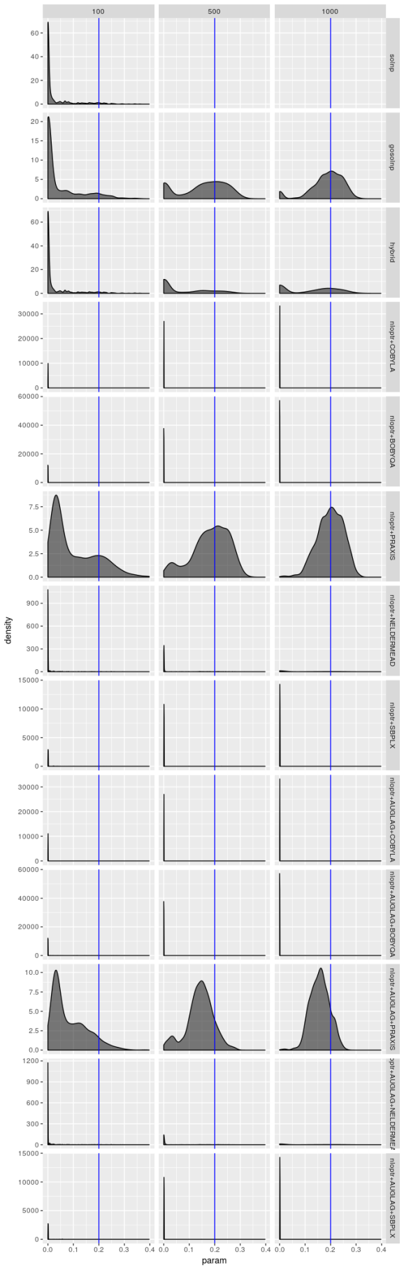
These tables already reveal a lot of information. In general it seems that the AUGLAG-PRAXIS method (the augmented Lagrangian method using the principal axis solver) provided in NLOpt does best for model 2 especially for large sample sizes, while for model 1 the gosolnp method, which uses the solnp solver by Yinyu Ye but with random initializations and restarts, seems to win out for larger sample sizes.
The bigger story, though, is the failure of any method to be the “best”, especially in the case of smaller sample sizes. While there are some optimizers that consistently fail to attain the maximum log-likelihood, no optimizer can claim to consistently obtain the best result. Additionally, different optimizers seem to perform better with different models. The implication for real-world data–where the true model parameters are never known–is to try every optimizer (or at least those that have a chance of maximizing the log-likelihood) and pick the results that yield the largest log-likelihood. No algorithm is trustworthy enough to be the go-to algorithm.
Let’s now look at plots of the estimated distribution of the parameters. First comes a helper function.
library(ggplot2)

solver_density_plot <- function(param, tags, list_reslist, sample_sizes, spec) {
  # Given a parameter, creates a density plot for each solver's distribution
  # at different sample sizes
  #
  # Args:
  #   param: A string for the parameter to plot
  #   tags: A character vector containing the solver names
  #   list_reslist: A list of lists created by optMethodSimsf, one for each
  #                 sample size
  #   sample_sizes: A numeric vector identifying the sample size corresponding
  #                 to each object in the above list
  #   spec: A ugarchspec object containing the specification that generated the
  #         datasets
  #
  # Returns:
  #   A ggplot object containing the plot generated

  p <- spec@model$fixed.pars[[param]]
  nlist <- lapply(list_reslist, function(l) {
    optlist <- lapply(tags, function(t) {
      return(na.omit(optMethodSims_getAllVals(param, t, l)))
    })
    names(optlist) <- tags
    df <- stack(optlist)
    names(df) <- c("param", "optimizer")

    return(df)
  })
  ndf <- do.call(rbind, nlist)
  ndf$n <- rep(sample_sizes, times = sapply(nlist, nrow))

  ggplot(ndf, aes(x = param)) + geom_density(fill = "black", alpha = 0.5) +
    geom_vline(xintercept = p, color = "blue") +
    facet_grid(optimizer ~ n, scales = "free_y")
}
Now for plots.
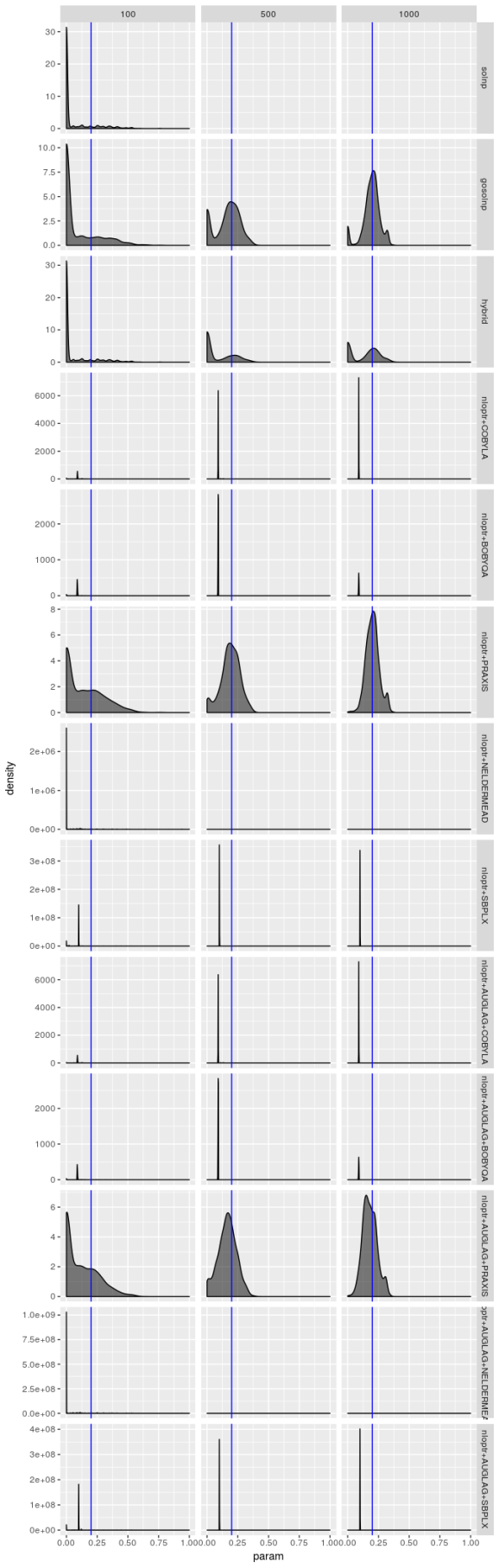
Estimated , model 1
solver_density_plot("omega", tags, list(spec1_n100, spec1_n500, spec1_n1000),
                    c(100, 500, 1000), spec1)
Estimated , model 1
solver_density_plot("alpha1", tags, list(spec1_n100, spec1_n500, spec1_n1000),
                    c(100, 500, 1000), spec1)
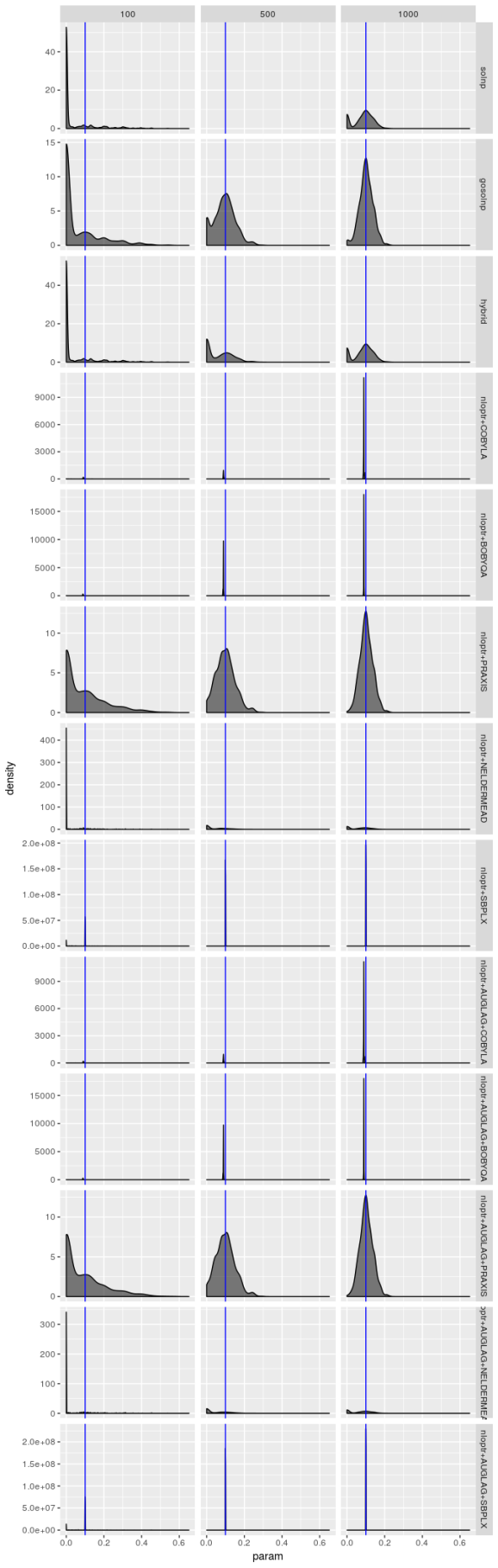
Estimated , model 1
solver_density_plot("beta1", tags, list(spec1_n100, spec1_n500, spec1_n1000),
                    c(100, 500, 1000), spec1)
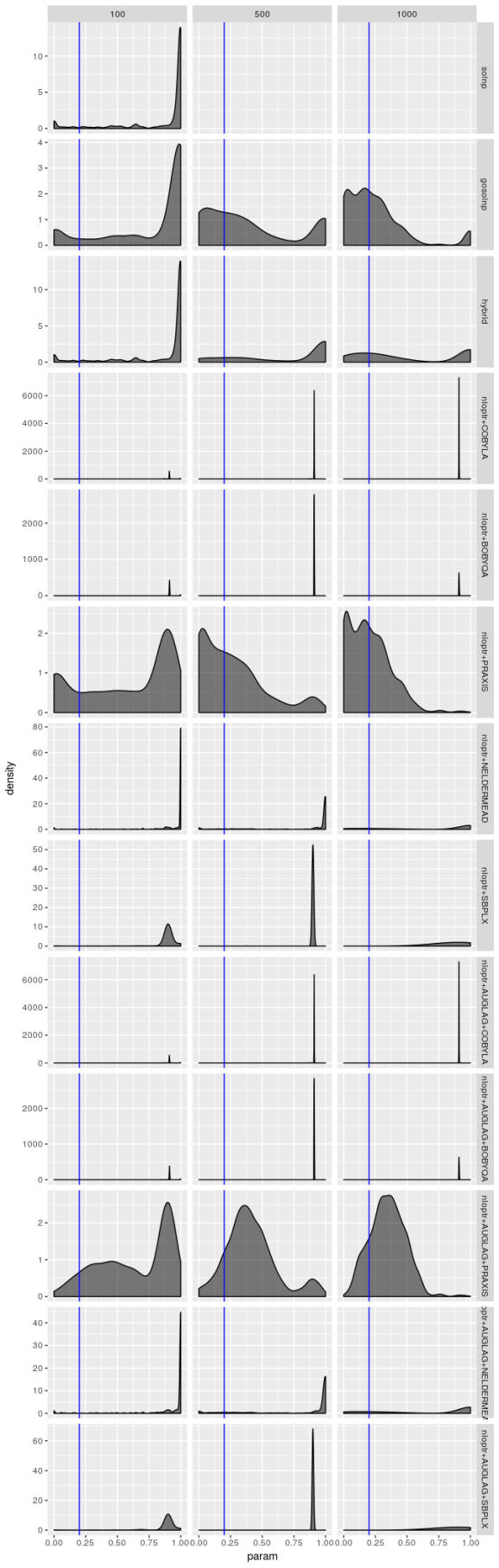
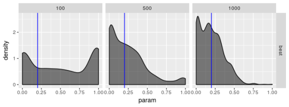
Bear in mind that there are only 1,000 simulated series and the optimizers produce solutions for each series, so in principle optimizer results should not be independent, yet the only time these density plots look the same is when the optimizer performs terribly. But even when an optimizer isn’t performing terribly (as is the case for the gosolnp, PRAXIS, and AUGLAG-PRAXIS methods) there’s evidence of artifacts around 0 for the estimates of AUGLAG-PRAXIS optimizer, though; it appears to produce biased estimates.
Let’s look at plots for model 2.
Estimated , model 2
solver_density_plot("omega", tags, list(spec2_n100, spec2_n500, spec2_n1000),
                    c(100, 500, 1000), spec2)

Estimated , model 2
solver_density_plot("alpha1", tags, list(spec2_n100, spec2_n500, spec2_n1000),
                    c(100, 500, 1000), spec2)
Estimated , model 2
solver_density_plot("beta1", tags, list(spec2_n100, spec2_n500, spec2_n1000),
                    c(100, 500, 1000), spec2)

The estimators don’t struggle as much for model 2, but the picture is still hardly rosy. The PRAXIS and AUGLAG-PRAXIS methods seem to perform well, but far from spectacularly for small sample sizes.
So far, my experiments suggest practitioners should not rely on any one optimizer but instead to try different ones and choose the results that have the largest log-likelihood. Suppose we call this optimization routine the “best” optimizer. how does this optimizer perform?
Let’s find out.
Model 1,
as.data.frame(round(solver_table(
  optMethodSims_getBestVals(spec1_n100, reslike = TRUE),
  "best", spec1) * 100,
  digits = 1))


##         Maximization Rate   Failure Rate   omega 95% CI Capture Rate   alpha1 95% CI Capture Rate   beta1 95% CI Capture Rate
## -----  ------------------  -------------  --------------------------  ---------------------------  --------------------------
## best                  100              0                        49.5                         63.3                        52.2
Model 1,
as.data.frame(round(solver_table(
  optMethodSims_getBestVals(spec1_n500, reslike = TRUE),
  "best", spec1) * 100,
  digits = 1))


##         Maximization Rate   Failure Rate   omega 95% CI Capture Rate   alpha1 95% CI Capture Rate   beta1 95% CI Capture Rate
## -----  ------------------  -------------  --------------------------  ---------------------------  --------------------------
## best                  100              0                          86                         88.8                        86.2
Model 1,
as.data.frame(round(solver_table(
  optMethodSims_getBestVals(spec1_n1000, reslike = TRUE),
  "best", spec1) * 100,
  digits = 1))


##         Maximization Rate   Failure Rate   omega 95% CI Capture Rate   alpha1 95% CI Capture Rate   beta1 95% CI Capture Rate
## -----  ------------------  -------------  --------------------------  ---------------------------  --------------------------
## best                  100              0                        92.8                         90.3                        92.4
Model 2,
as.data.frame(round(solver_table(
  optMethodSims_getBestVals(spec2_n100, reslike = TRUE),
  "best", spec2) * 100,
  digits = 1))


##         Maximization Rate   Failure Rate   omega 95% CI Capture Rate   alpha1 95% CI Capture Rate   beta1 95% CI Capture Rate
## -----  ------------------  -------------  --------------------------  ---------------------------  --------------------------
## best                  100              0                        55.2                         63.2                        52.2
Model 2,
as.data.frame(round(solver_table(
  optMethodSims_getBestVals(spec2_n500, reslike = TRUE),
  "best", spec2) * 100,
  digits = 1))


##         Maximization Rate   Failure Rate   omega 95% CI Capture Rate   alpha1 95% CI Capture Rate   beta1 95% CI Capture Rate
## -----  ------------------  -------------  --------------------------  ---------------------------  --------------------------
## best                  100              0                          83                         86.3                        80.5
Model 2,
as.data.frame(round(solver_table(
  optMethodSims_getBestVals(spec2_n1000, reslike = TRUE),
  "best", spec2) * 100,
  digits = 1))


##         Maximization Rate   Failure Rate   omega 95% CI Capture Rate   alpha1 95% CI Capture Rate   beta1 95% CI Capture Rate
## -----  ------------------  -------------  --------------------------  ---------------------------  --------------------------
## best                  100              0                        88.7                         91.4                        88.1
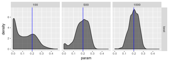
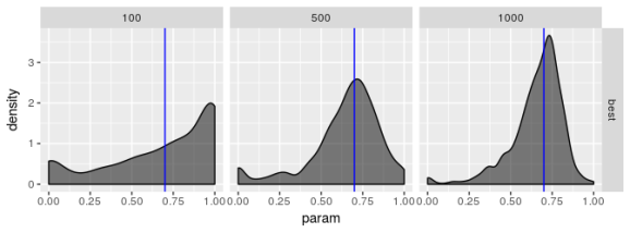
Bear in mind that we evaluate the performance of the “best” optimizer by the CI capture rate, which should be around 95%. The “best” optimizer obviously has good performance but does not outperform all optimizers. This is disappointing; I had hoped that the “best” optimizer would have the highly desirable property of a 95% capture rate. Performance is nowhere near that except for larger sample sizes. Either the standard errors are being underestimated or for small sample sizes the Normal distribution poorly describes the actual distribution of the estimators (which means multiplying by two does not lead to intervals with the desired confidence level).
Interestingly, there is no noticeable difference in performance between the two models for this “best” estimator. This suggests to me that the seemingly better results for models often seen in actual data might be exploiting the bias of the optimizers.
Let’s look at the distribution of the estimated parameters.
Estimated , model 1
solver_density_plot("omega", "best",
                    lapply(list(spec1_n100, spec1_n500, spec1_n1000),
                           function(l) {optMethodSims_getBestVals(l,
                                                              reslike = TRUE)}),
                    c(100, 500, 1000), spec1)
Estimated , model 1
solver_density_plot("alpha1", "best",
                    lapply(list(spec1_n100, spec1_n500, spec1_n1000),
                           function(l) {optMethodSims_getBestVals(l,
                                                              reslike = TRUE)}),
                    c(100, 500, 1000), spec1)

Estimated , model 1
solver_density_plot("beta1", "best",
                    lapply(list(spec1_n100, spec1_n500, spec1_n1000),
                           function(l) {optMethodSims_getBestVals(l,
                                                              reslike = TRUE)}),
                    c(100, 500, 1000), spec1)
Estimated , model 2
solver_density_plot("omega", "best",
                    lapply(list(spec2_n100, spec2_n500, spec2_n1000),
                           function(l) {optMethodSims_getBestVals(l,
                                                              reslike = TRUE)}),
                    c(100, 500, 1000), spec2)

Estimated , model 2
solver_density_plot("alpha1", "best",
                    lapply(list(spec2_n100, spec2_n500, spec2_n1000),
                           function(l) {optMethodSims_getBestVals(l,
                                                              reslike = TRUE)}),
                    c(100, 500, 1000), spec2)

Estimated , model 2
solver_density_plot("beta1", "best",
                    lapply(list(spec2_n100, spec2_n500, spec2_n1000),
                           function(l) {optMethodSims_getBestVals(l,
                                                              reslike = TRUE)}),
                    c(100, 500, 1000), spec2)
The plots suggest that the “best” estimator still shows some pathologies even though it behaves less poorly than the other estimators. I don’t see evidence for bias in parameter estimates regardless of choice of model but I’m not convinced the “best” estimator truly maximizes the log-likelihood, especially for smaller sample sizes. the estimates for
Conclusion
I initially wrote this article over a year ago and didn’t publish it until now. The reason for the hang up was because I wanted a literature review of alternative ways to estimate the parameters of a GARCH model. Unfortunately I never completed such a review, and I’ve decided to release this article regardless.
That said, I’ll share what I was reading. One article by Gilles Zumbach tried to explain why estimating GARCH parameters is hard. He noted that the quasi-likelihood equation that solvers try to maximize has bad properties, such as being non-concave and having “flat” regions that algorithms can become stuck in. He suggested an alternative procedure to finding the parameters of GARCH models, where one finds the best fit in an alternative parameter space (which supposedly has better properties than working with the original parameter space of GARCH models) and estimating one of the parameters using, say, the method of moments, without any optimization algorithm. Another article, by Fiorentini, Calzolari, and Panattoni, showed that analytic gradients for GARCH models could be computed explicitly, so gradient-free methods like those used by the optimization algorithms seen here are not actually necessary. Since numerical differentiation is generally a difficult problem, this could help ensure that no additional numerical error is being introduced that causes these algorithms to fail to converge. I also wanted to explore other estimation methods to see if they somehow can avoid numerical techniques altogether or have better numerical properties, such as estimation via method of moments. I wanted to read an article by Andersen, Chung, and Sørensen to learn more about this approach to estimation.
Life happens, though, and I didn’t complete this review. The project moved on and the problem of estimating GARCH model parameters well was essentially avoided. That said, I want to revisit this point, perhaps exploring how techniques such as simulated annealing do for estimating GARCH model parameters.
So for now, if you’re a practitioner, what should you do when estimating a GARCH model? I would say don’t take for granted that the default estimation procedure your package uses will work. You should explore different procedure and different parameter choices and go with the results that lead to the largest log-likelihood value. I showed how this could be done in an automated fashion but you should be prepared to manually pick the model with the best fit (as determined by the log-likelihood). If you don’t do this the model you estimated may not actually be the one for which theory works.
I will say it again, one last time, in the last sentence of this article for extra emphasis: don’t take numerical techniques and results for granted!
sessionInfo()


## R version 3.4.2 (2017-09-28)
## Platform: i686-pc-linux-gnu (32-bit)
## Running under: Ubuntu 16.04.2 LTS
##
## Matrix products: default
## BLAS: /usr/lib/libblas/libblas.so.3.6.0
## LAPACK: /usr/lib/lapack/liblapack.so.3.6.0
##
## locale:
##  [1] LC_CTYPE=en_US.UTF-8       LC_NUMERIC=C
##  [3] LC_TIME=en_US.UTF-8        LC_COLLATE=en_US.UTF-8
##  [5] LC_MONETARY=en_US.UTF-8    LC_MESSAGES=en_US.UTF-8
##  [7] LC_PAPER=en_US.UTF-8       LC_NAME=C
##  [9] LC_ADDRESS=C               LC_TELEPHONE=C
## [11] LC_MEASUREMENT=en_US.UTF-8 LC_IDENTIFICATION=C
##
## attached base packages:
## [1] parallel  stats     graphics  grDevices utils     datasets  methods
## [8] base
##
## other attached packages:
## [1] ggplot2_2.2.1 rugarch_1.3-8 printr_0.1
##
## loaded via a namespace (and not attached):
##  [1] digest_0.6.16               htmltools_0.3.6
##  [3] SkewHyperbolic_0.3-2        expm_0.999-2
##  [5] scales_0.5.0                DistributionUtils_0.5-1
##  [7] Rsolnp_1.16                 rprojroot_1.2
##  [9] grid_3.4.2                  stringr_1.3.1
## [11] knitr_1.17                  numDeriv_2016.8-1
## [13] GeneralizedHyperbolic_0.8-1 munsell_0.4.3
## [15] pillar_1.3.0                tibble_1.4.2
## [17] compiler_3.4.2              highr_0.6
## [19] lattice_0.20-35             labeling_0.3
## [21] Matrix_1.2-8                KernSmooth_2.23-15
## [23] plyr_1.8.4                  xts_0.10-0
## [25] spd_2.0-1                   zoo_1.8-0
## [27] stringi_1.2.4               magrittr_1.5
## [29] reshape2_1.4.2              rlang_0.2.2
## [31] rmarkdown_1.7               evaluate_0.10.1
## [33] gtable_0.2.0                colorspace_1.3-2
## [35] yaml_2.1.14                 tools_3.4.2
## [37] mclust_5.4.1                mvtnorm_1.0-6
## [39] truncnorm_1.0-7             ks_1.11.3
## [41] nloptr_1.0.4                lazyeval_0.2.1
## [43] crayon_1.3.4                backports_1.1.1
## [45] Rcpp_1.0.0
Packt Publishing published a book for me entitled Hands-On Data Analysis with NumPy and Pandas, a book based on my video course Unpacking NumPy and Pandas. This book covers the basics of setting up a Python environment for data analysis with Anaconda, using Jupyter notebooks, and using NumPy and pandas. If you are starting out using Python for data analysis or know someone who is, please consider buying my book or at least spreading the word about it. You can buy the book directly or purchase a subscription to Mapt and read it there.
If you like my blog and would like to support it, spread the word (if not get a copy yourself)!
-
When I wrote this article initially, my advisor and a former student of his developed a test statistic that should detect early or late change points in a time series, including a change in the parameters of a GARCH model. My contribution to the paper we were writing included demonstrating that the test statistic detects structural change sooner than other test statistics when applied to real-world data. To be convincing to reviewers, our test statistic should detect a change that another statistic won’t detect until getting more data. This means that the change should be present but not so strong that both statistics immediately detect the change with miniscule
-values. ↩
- The profile on LinkedIn I linked to may or may not be the correct person; I’m guessing it is based on the listed occupations and history. If I got the wrong person, I’m sorry. ↩
R-bloggers.com offers daily e-mail updates about R news and tutorials about learning R and many other topics. Click here if you're looking to post or find an R/data-science job.
Want to share your content on R-bloggers? click here if you have a blog, or here if you don't.