
One-arm Bayesian Adaptive Trial Simulation Code
[This article was first published on R – BioStatMatt, and kindly contributed to R-bloggers]. (You can report issue about the content on this page here)
Want to share your content on R-bloggers? click here if you have a blog, or here if you don't.
Want to share your content on R-bloggers? click here if you have a blog, or here if you don't.
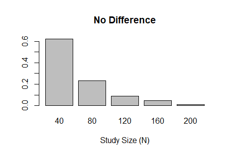
I had an opportunity recently to design a Bayesian adaptive trial with several interim analyses that allow for early stopping due to efficacy or futility. The code below implements the one-arm trial described in the great introductory article by Ben Saville et al. Three of the coauthors are current or former colleagues at Vandy. The figures below the code show the sample size distribution under the null hypothesis and an alternative hypothesis, respectively.
## Simulate Bayesian single-arm adaptive trial
## Allow early termination due to futility or efficacy
## Binary outcome
## Beta-binomial:
##   p   ~ beta(a, b)
##   x_i ~ binomial(p)  i = 1..n
##   p|x ~ beta(a + sum(x), b + n - sum(x))
## Efficacy at interim t if Pr(p > p_0 | x_{(t)}) > \gamma_e
## Futility at interim t if Pr(p > p_0 | x_{(t_max)}) < \gamma_f
## https://www.ncbi.nlm.nih.gov/pmc/articles/PMC4247348/

library('rmutil') ## for betabinom
## Simulate entire trial
## ptru - true probability of outcome (p)
## pref - reference probability of outcome (p_0)
## nint - sample sizes at which to conduct interim analyses
## efft - efficacy threshold
## futt - futility threshold
## apri - prior beta parameter \alpha
## bpri - prior beta parameter \beta
simtrial <- function(
  ptru = 0.15,
  pref = 0.15,
  nint = c(10, 13, 16, 19),
  efft = 0.95,
  futt = 0.05,
  apri = 1,
  bpri = 1) {

  ## determine minimum number of 'successes' necessary to
  ## conclude efficacy if study continues to maximum
  ## sample size
  nmax <- max(nint)
  post <- sapply(0:nmax, function(nevt)
    1-pbeta(pref, apri + nevt, bpri + nmax - nevt))
  nsuc <- min(which(post > efft)-1)


  ## simulate samples
  samp <- rbinom(n = nmax, size = 1, prob = ptru)

  ## simulate interim analyses
  intr <- lapply(nint, function(ncur) {

    ## compute number of current events
    ecur <- sum(samp[1:ncur])

    ## compute posterior beta parameters
    abb <- apri + ecur
    bbb <- bpri + ncur - ecur
    sbb <- abb + bbb
    mbb <- abb/(abb+bbb)

    ## compute efficacy Pr(p > p_0 | x_{(t)})
    effp <- 1-pbeta(pref, abb, bbb)

    ## return for efficacy
    if(effp > efft)
      return(list(action='stop',
                  reason='efficacy',
                  n = ncur))

    ## number of events necessary in remainder of
    ## study to conclude efficacy
    erem <- nsuc-ecur

    ## compute success probability Pr(p > p_0 | x_{(t_max)})
    if(erem > nmax-ncur) { ## not enough possible events
      sucp <- 0
    } else { ## not yet met efficacy threshold
      sucp <- 1-pbetabinom(q = erem-1,
        size = nmax-ncur, m = mbb, s = sbb)
    }

    if(sucp < futt)
      return(list(action='stop',
                  reason='futility',
                  n = ncur))

    return(list(action='continue',
                reason='',
                n = ncur))
  })

  stpi <- match('stop', sapply(intr, `[[`, 'action'))
  return(intr[[stpi]])
}


## Simulate study with max sample size of 200 where true
## probability is identical to reference (i.e., the null
## hypothesis is true). This type of simulation helps us
## determine the overall type-I error rate.
nint <- c(40,80,120,160,200)
nmax <- max(nint)
res <- do.call(rbind, lapply(1:10000,
  function(t) as.data.frame(simtrial(ptru = 0.72,
                                     pref = 0.72,
                                     nint = nint,
                                     efft = 0.975,
                                     futt = 0.20))))

## Prob. early termination (PET) due to Futility
mean(res$reason == 'futility' & res$n < nmax)
## PET Efficacy
mean(res$reason == 'efficacy' & res$n < nmax)
## Pr(conclude efficacy) 'type-I error rate'
mean(res$reason == 'efficacy')
## average and sd sample size
mean(res$n); sd(res$n)
barplot(prop.table(table(res$n)),
        xlab='Study Size (N)',
        main="No Difference")

## Simulate study where true probability is greater than
## reference (i.e., an alternative hypothesis). This type
## of simulation helps us determine the study power.
res <- do.call(rbind, lapply(1:10000,
  function(t) as.data.frame(simtrial(ptru = 0.82,
                                     pref = 0.72,
                                     nint = nint,
                                     efft = 0.975,
                                     futt = 0.20))))

## Prob. early termination (PET) due to Futility
mean(res$reason == 'futility' & res$n < nmax)
## PET Efficacy
mean(res$reason == 'efficacy' & res$n < nmax)
## Pr(conclude efficacy) 'power'
mean(res$reason == 'efficacy')
## average and sd sample size
mean(res$n); sd(res$n)
barplot(prop.table(table(res$n)),
        xlab='Study Size (N)',
        main="35% Reduction")

To leave a comment for the author, please follow the link and comment on their blog: R – BioStatMatt.
R-bloggers.com offers daily e-mail updates about R news and tutorials about learning R and many other topics. Click here if you're looking to post or find an R/data-science job.
Want to share your content on R-bloggers? click here if you have a blog, or here if you don't.