Convert from MetaLandSim to igraph

Then, we should get a data frame with the data (here, the MetaLandSim sample data):

data(mc_df)

Then, convert to a ‘metapopulation’ class object (beware of the column order, check MetaLandSim manual)

sp1 <- convert.graph(dframe=mc_df, mapsize=8300, dispersal=800)
#head(sp1$nodes.characteristics)#check the head of the table

Now, remove species presence/absence information:

rl1 <- remove.species(sp=sp1)

Next, create a table with the nodes information:

df1 <- rl1$nodes.characteristics
df2 <- cbind(df1$ID, df1[,-8]) # change the columns order
names(df2)[1] <- "ID" #rename ID column

Almost finished… Now, to get data frame with the edges details:

edge_df <- edge.graph(rl=rl1)
head(edge_df) #check the top of the table
##   ID node A node B area ndA area ndB       XA      YA       XB YB
## 1  1      2      1    0.781    0.079 1420.857  46.725 1248.254  0
## 2  2      3      1    1.053    0.079 1278.912  52.629 1248.254  0
## 3  3      5      1    0.079    0.079 1151.337  97.140 1248.254  0
## 4  4      6      1    0.137    0.079 1295.796 104.839 1248.254  0
## 5  5      7      1    0.013    0.079  855.687 110.980 1248.254  0
## 6  6     10      1    0.154    0.079 1367.670 154.928 1248.254  0
##    distance
## 1 178.81561
## 2  60.90751
## 3 137.21911
## 4 115.11498
## 5 407.95271
## 6 195.60896

And finally, create igraph object:

g1 <- graph.data.frame(d=edge_df[,-1], directed=FALSE, vertices=df2)

Let’s plot it (it’s a bit messy! too much vertexes):

Convert from igraph to MetaLandSim

Now, having g1, the igraph object we previously created, we will obtain a ‘landscape’ class object (from the package MetaLandSim).

First, convert the igraph graph to a data frame:

df3 <- as_long_data_frame(g1)#each row is an edge

But… we want a data frame in which each row is an node (or vertex in igraph nomenclature). And here each row is an edge (a connection).

So…

l1 <- vertex_attr(g1, index = V(g1))#getting a list of attributes

But… check out the structure (using ‘str’) of this object! In this list each element is an attribute. That’s not what we need exactly!

So…we create the desired data frame, by de-constructing the list:

df3 <- data.frame(matrix(unlist(l1), nrow=length(l1[[1]]), byrow=FALSE),stringsAsFactors=FALSE)
names(df3) <- names (l1)
head(df3)
##   name        x       y areas           radius cluster    colour
## 1    1 1248.254       0 0.079 15.8576420089872       1 #FF0000FF
## 2    2 1420.857  46.725 0.781 49.8598055661613       1 #FF0000FF
## 3    3 1278.912  52.629 1.053 57.8947588432262       1 #FF0000FF
## 4    4 6370.625  62.637 0.788 50.0827505547396       1 #FF0000FF
## 5    5 1151.337   97.14 0.079 15.8576420089872       1 #FF0000FF
## 6    6 1295.796 104.839 0.137 20.8826373830461       1 #FF0000FF
##         nneighbour
## 1 60.9075086093661
## 2 120.568429441542
## 3 54.8721564730237
## 4 262.650432704765
## 5 133.177624186648
## 6 54.8721564730237

But MetaLandSim requires a specific column order (see MetaLandSim manual for details):

df4 <- cbind(as.numeric(df3$name), as.numeric(df3$x), as.numeric(df3$y), as.numeric(df3$areas), 0)

(Note that I needed to use ‘as.numeric’ to convert all columns from character to numeric.)

And now, from data frame to ‘landscape’ object (we’re almost there!):

rl2 <- convert.graph(dframe=df4, mapsize=8300, dispersal=800)

Finally! Remove the species:

rl2 <- remove.species(sp=rl2)

Plot side by side (the MetaLandSim graph we got, after transforming it from igraph, and the original MetaLandSim graph):

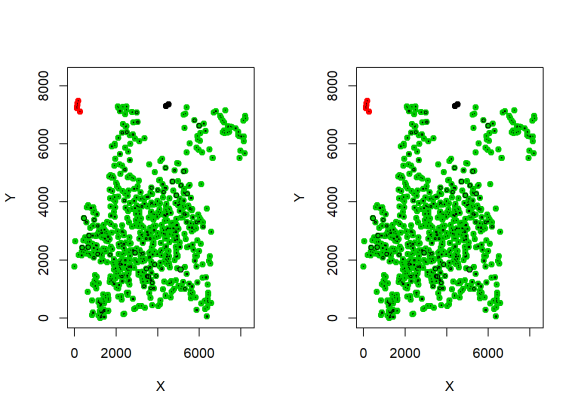
The graphs are the equal. No surprise there, that’s what they’re suppose to be!!

I know… this is harder than it should be!

In my defense I can say that MetaLandSim was never intended to be used like this. However, of course, other users have their own requirements and work flows.

I hope this was helpful!