
Deep Learning from first principles in Python, R and Octave – Part 6
Want to share your content on R-bloggers? click here if you have a blog, or here if you don't.
“Today you are You, that is truer than true. There is no one alive who is Youer than You.”
Dr. Seuss
“Explanations exist; they have existed for all time; there is always a well-known solution to every human problem — neat, plausible, and wrong.”
H L Mencken
Introduction
In this 6th instalment of ‘Deep Learning from first principles in Python, R and Octave-Part6’, I look at a couple of different initialization techniques used in Deep Learning, L2 regularization and the ‘dropout’ method. Specifically, I implement “He initialization” & “Xavier Initialization”. My earlier posts in this series of Deep Learning included
1. Part 1 – In the 1st part, I implemented logistic regression as a simple 2 layer Neural Network
2. Part 2 – In part 2, implemented the most basic of Neural Networks, with just 1 hidden layer, and any number of activation units in that hidden layer. The implementation was in vectorized Python, R and Octave
3. Part 3 -In part 3, I derive the equations and also implement a L-Layer Deep Learning network with either the relu, tanh or sigmoid activation function in Python, R and Octave. The output activation unit was a sigmoid function for logistic classification
4. Part 4 – This part looks at multi-class classification, and I derive the Jacobian of a Softmax function and implement a simple problem to perform multi-class classification.
5. Part 5 – In the 5th part, I extend the L-Layer Deep Learning network implemented in Part 3, to include the Softmax classification. I also use this L-layer implementation to classify MNIST handwritten digits with Python, R and Octave.
The code in Python, R and Octave are identical, and just take into account some of the minor idiosyncrasies of the individual language. In this post, I implement different initialization techniques (random, He, Xavier), L2 regularization and finally dropout. Hence my generic L-Layer Deep Learning network includes these additional enhancements for enabling/disabling initialization methods, regularization or dropout in the algorithm. It already included sigmoid & softmax output activation for binary and multi-class classification, besides allowing relu, tanh and sigmoid activation for hidden units.
This R Markdown file and the code for Python, R and Octave can be cloned/downloaded from Github at DeepLearning-Part6
1. Initialization techniques
The usual initialization technique is to generate Gaussian or uniform random numbers and multiply it by a small value like 0.01. Two techniques which are used to speed up convergence is the He initialization or Xavier. These initialization techniques enable gradient descent to converge faster.
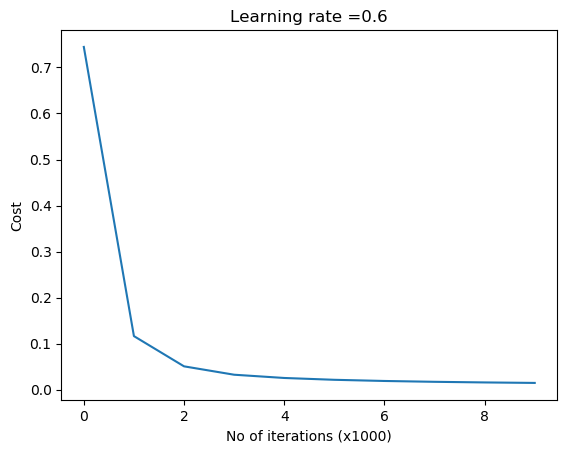
1.1 a Default initialization – Python
This technique just initializes the weights to small random values based on Gaussian or uniform distribution
import numpy as np
import matplotlib
import matplotlib.pyplot as plt
import sklearn.linear_model
import pandas as pd
import sklearn
import sklearn.datasets
exec(open("DLfunctions61.py").read())
#Load the data
train_X, train_Y, test_X, test_Y = load_dataset()
# Set the layers dimensions
layersDimensions = [2,7,1]
# Train a deep learning network with random initialization
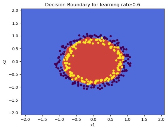
parameters = L_Layer_DeepModel(train_X, train_Y, layersDimensions, hiddenActivationFunc='relu', outputActivationFunc="sigmoid",learningRate = 0.6, num_iterations = 9000, initType="default", print_cost = True,figure="fig1.png")
# Clear the plot
plt.clf()
plt.close()
# Plot the decision boundary
plot_decision_boundary(lambda x: predict(parameters, x.T), train_X, train_Y,str(0.6),figure1="fig2.png")


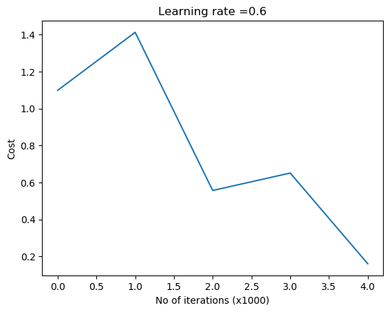
1.1 b He initialization – Python
‘He’ initialization attributed to He et al, multiplies the random weights by

import numpy as np
import matplotlib
import matplotlib.pyplot as plt
import sklearn.linear_model
import pandas as pd
import sklearn
import sklearn.datasets
exec(open("DLfunctions61.py").read())
#Load the data
train_X, train_Y, test_X, test_Y = load_dataset()
# Set the layers dimensions
layersDimensions = [2,7,1]
# Train a deep learning network with He initialization
parameters = L_Layer_DeepModel(train_X, train_Y, layersDimensions, hiddenActivationFunc='relu', outputActivationFunc="sigmoid", learningRate =0.6, num_iterations = 10000,initType="He",print_cost = True, figure="fig3.png")
plt.clf()
plt.close()
# Plot the decision boundary
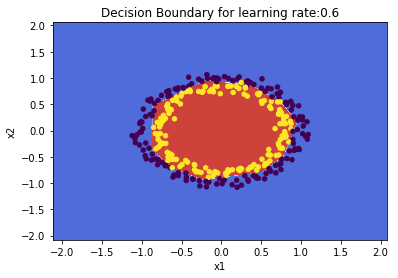
plot_decision_boundary(lambda x: predict(parameters, x.T), train_X, train_Y,str(0.6),figure1="fig4.png")
1.1 c Xavier initialization – Python
Xavier initialization multiply the random weights by

import numpy as np
import matplotlib
import matplotlib.pyplot as plt
import sklearn.linear_model
import pandas as pd
import sklearn
import sklearn.datasets
exec(open("DLfunctions61.py").read())

#Load the data
train_X, train_Y, test_X, test_Y = load_dataset()
# Set the layers dimensions
layersDimensions = [2,7,1]

# Train a L layer Deep Learning network
parameters = L_Layer_DeepModel(train_X, train_Y, layersDimensions, hiddenActivationFunc='relu', outputActivationFunc="sigmoid",
                            learningRate = 0.6,num_iterations = 10000, initType="Xavier",print_cost = True,
                            figure="fig5.png")

# Plot the decision boundary
plot_decision_boundary(lambda x: predict(parameters, x.T), train_X, train_Y,str(0.6),figure1="fig6.png")


1.2a Default initialization – R
source("DLfunctions61.R")
#Load the data
z <- as.matrix(read.csv("circles.csv",header=FALSE))
x <- z[,1:2]
y <- z[,3]
X <- t(x)
Y <- t(y)
#Set the layer dimensions
layersDimensions = c(2,11,1)
# Train a deep learning network
retvals = L_Layer_DeepModel(X, Y, layersDimensions,
                            hiddenActivationFunc='relu',
                            outputActivationFunc="sigmoid",
                            learningRate = 0.5,
                            numIterations = 9000,
                            initType="default",
                            print_cost = True)
#Plot the cost vs iterations
iterations <- seq(0,9000,1000)
costs=retvals$costs
df=data.frame(iterations,costs)
ggplot(df,aes(x=iterations,y=costs)) + geom_point() + geom_line(color="blue") +
 ggtitle("Costs vs iterations") + xlab("No of iterations") + ylab("Cost")

# Plot the decision boundary
plotDecisionBoundary(z,retvals,hiddenActivationFunc="relu",lr=0.5)

1.2b He initialization – R
source("DLfunctions61.R")
# Load the data
z <- as.matrix(read.csv("circles.csv",header=FALSE))
x <- z[,1:2]
y <- z[,3]
X <- t(x)
Y <- t(y)
# Set the layer dimensions
layersDimensions = c(2,11,1)
# Train a deep learning network
retvals = L_Layer_DeepModel(X, Y, layersDimensions,
                            hiddenActivationFunc='relu',
                            outputActivationFunc="sigmoid",
                            learningRate = 0.5,
                            numIterations = 9000,
                            initType="He",
                            print_cost = True)
#Plot the cost vs iterations
iterations <- seq(0,9000,1000)
costs=retvals$costs
df=data.frame(iterations,costs)
ggplot(df,aes(x=iterations,y=costs)) + geom_point() + geom_line(color="blue") +
    ggtitle("Costs vs iterations") + xlab("No of iterations") + ylab("Cost")

# Plot the decision boundary
plotDecisionBoundary(z,retvals,hiddenActivationFunc="relu",0.5,lr=0.5)

1.2c Xavier initialization – R
## Xav initialization
# Set the layer dimensions
layersDimensions = c(2,11,1)
# Train a deep learning network
retvals = L_Layer_DeepModel(X, Y, layersDimensions,
                            hiddenActivationFunc='relu',
                            outputActivationFunc="sigmoid",
                            learningRate = 0.5,
                            numIterations = 9000,
                            initType="Xav",
                            print_cost = True)
#Plot the cost vs iterations
iterations <- seq(0,9000,1000)
costs=retvals$costs
df=data.frame(iterations,costs)
ggplot(df,aes(x=iterations,y=costs)) + geom_point() + geom_line(color="blue") +
    ggtitle("Costs vs iterations") + xlab("No of iterations") + ylab("Cost")

# Plot the decision boundary
plotDecisionBoundary(z,retvals,hiddenActivationFunc="relu",0.5)

1.3a Default initialization – Octave
source("DL61functions.m")
# Read the data
data=csvread("circles.csv");

X=data(:,1:2);
Y=data(:,3);
# Set the layer dimensions
layersDimensions = [2 11  1]; #tanh=-0.5(ok), #relu=0.1 best!

# Train a deep learning network
[weights biases costs]=L_Layer_DeepModel(X', Y', layersDimensions,
                               hiddenActivationFunc='relu',
                               outputActivationFunc="sigmoid",
                               learningRate = 0.5,
                               lambd=0,
                               keep_prob=1,
                               numIterations = 10000,
                               initType="default");
# Plot cost vs iterations
plotCostVsIterations(10000,costs)
#Plot decision boundary
plotDecisionBoundary(data,weights, biases,keep_prob=1, hiddenActivationFunc="relu")


1.3b He initialization – Octave
source("DL61functions.m")
#Load data
data=csvread("circles.csv");
X=data(:,1:2);
Y=data(:,3);
# Set the layer dimensions
layersDimensions = [2 11  1]; #tanh=-0.5(ok), #relu=0.1 best!

# Train a deep learning network
[weights biases costs]=L_Layer_DeepModel(X', Y', layersDimensions,
                               hiddenActivationFunc='relu',
                               outputActivationFunc="sigmoid",
                               learningRate = 0.5,
                               lambd=0,
                               keep_prob=1,
                               numIterations = 8000,
                               initType="He");
plotCostVsIterations(8000,costs)
#Plot decision boundary
plotDecisionBoundary(data,weights, biases,keep_prob=1,hiddenActivationFunc="relu")


1.3c Xavier initialization – Octave
source("DL61functions.m")
#Load data
data=csvread("circles.csv");
X=data(:,1:2);
Y=data(:,3);
#Set layer dimensions
layersDimensions = [2 11  1]; #tanh=-0.5(ok), #relu=0.1 best!

# Train a deep learning network
[weights biases costs]=L_Layer_DeepModel(X', Y', layersDimensions,
                               hiddenActivationFunc='relu',
                               outputActivationFunc="sigmoid",
                               learningRate = 0.5,
                               lambd=0,
                               keep_prob=1,
                               numIterations = 8000,
                               initType="Xav");

plotCostVsIterations(8000,costs)
plotDecisionBoundary(data,weights, biases,keep_prob=1,hiddenActivationFunc="relu")


2.1a Regularization : Circles data – Python
The cross entropy cost for Logistic classification is given as
^{(i)}) - (1-y^{i})log((a^{L})^{(i)})")
The regularized L2 cost is given by
^{(i)}) - (1-y^{i})log((a^{L})^{(i)}) + \frac{\lambda}{2m}\sum \sum \sum W_{kj}^{l}")
Incidentally, a detailed implementation of L1 and L2 regularization in Machine Learning, besides other feature selection methods can be found in my book ‘Practical Machine Learning with R and Python: Machine Learning in stereo‘ available in Amazon. My book is compact and can be used as a quick reference for ML algorithms and associated metrics

import numpy as np
import matplotlib
import matplotlib.pyplot as plt
import sklearn.linear_model
import pandas as pd
import sklearn
import sklearn.datasets
exec(open("DLfunctions61.py").read())

#Load the data
train_X, train_Y, test_X, test_Y = load_dataset()
# Set the layers dimensions
layersDimensions = [2,7,1]

# Train a deep learning network
parameters = L_Layer_DeepModel(train_X, train_Y, layersDimensions, hiddenActivationFunc='relu',
                               outputActivationFunc="sigmoid",learningRate = 0.6, lambd=0.1, num_iterations = 9000,
                               initType="default", print_cost = True,figure="fig7.png")

# Clear the plot
plt.clf()
plt.close()

# Plot the decision boundary
plot_decision_boundary(lambda x: predict(parameters, x.T), train_X, train_Y,str(0.6),figure1="fig8.png")


plt.clf()
plt.close()
#Plot the decision boundary
plot_decision_boundary(lambda x: predict(parameters, x.T,keep_prob=0.9), train_X, train_Y,str(2.2),"fig8.png",)

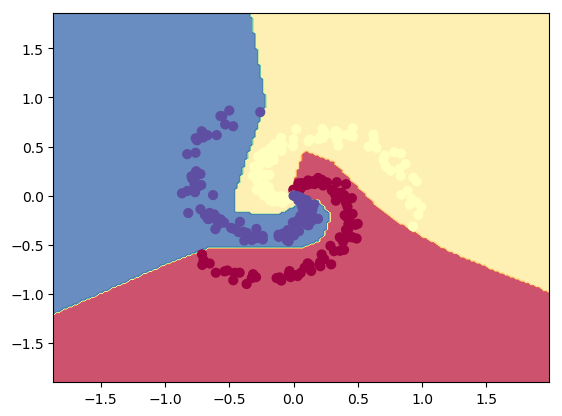
2.1 b Regularization: Spiral data – Python
import numpy as np
import matplotlib
import matplotlib.pyplot as plt
import sklearn.linear_model
import pandas as pd
import sklearn
import sklearn.datasets
exec(open("DLfunctions61.py").read())
N = 100 # number of points per class
D = 2 # dimensionality
K = 3 # number of classes
X = np.zeros((N*K,D)) # data matrix (each row = single example)
y = np.zeros(N*K, dtype='uint8') # class labels
for j in range(K):
  ix = range(N*j,N*(j+1))
  r = np.linspace(0.0,1,N) # radius
  t = np.linspace(j*4,(j+1)*4,N) + np.random.randn(N)*0.2 # theta
  X[ix] = np.c_[r*np.sin(t), r*np.cos(t)]
  y[ix] = j


# Plot the data
plt.scatter(X[:, 0], X[:, 1], c=y, s=40, cmap=plt.cm.Spectral)
plt.clf()
plt.close()
#Set layer dimensions
layersDimensions = [2,100,3]
y1=y.reshape(-1,1).T
# Train a deep learning network
parameters = L_Layer_DeepModel(X.T, y1, layersDimensions, hiddenActivationFunc='relu', outputActivationFunc="softmax",
                           learningRate = 0.6,lambd=0.2, num_iterations = 5000, print_cost = True,figure="fig9.png")

plt.clf()
plt.close()
W1=parameters['W1']
b1=parameters['b1']
W2=parameters['W2']
b2=parameters['b2']
plot_decision_boundary1(X, y1,W1,b1,W2,b2,figure2="fig10.png")


2.2a Regularization: Circles data – R
source("DLfunctions61.R")
#Load data
df=read.csv("circles.csv",header=FALSE)
z <- as.matrix(read.csv("circles.csv",header=FALSE))
x <- z[,1:2]
y <- z[,3]
X <- t(x)
Y <- t(y)
#Set layer dimensions
layersDimensions = c(2,11,1)
# Train a deep learning network
retvals = L_Layer_DeepModel(X, Y, layersDimensions,
                            hiddenActivationFunc='relu',
                            outputActivationFunc="sigmoid",
                            learningRate = 0.5,
                            lambd=0.1,
                            numIterations = 9000,
                            initType="default",
                            print_cost = True)

#Plot the cost vs iterations
iterations <- seq(0,9000,1000)
costs=retvals$costs
df=data.frame(iterations,costs)
ggplot(df,aes(x=iterations,y=costs)) + geom_point() + geom_line(color="blue") +
    ggtitle("Costs vs iterations") + xlab("No of iterations") + ylab("Cost")

# Plot the decision boundary
plotDecisionBoundary(z,retvals,hiddenActivationFunc="relu",0.5)

2.2b Regularization:Spiral data – R
# Read the spiral dataset
#Load the data
source("DLfunctions61.R")
Z <- as.matrix(read.csv("spiral.csv",header=FALSE))

# Setup the data
X <- Z[,1:2]
y <- Z[,3]
X <- t(X)
Y <- t(y)

layersDimensions = c(2, 15, 6, 3)
# Train a deep learning network
retvals = L_Layer_DeepModel(X, Y, layersDimensions,
                            hiddenActivationFunc='relu',
                            outputActivationFunc="softmax",
                            learningRate = 5.1,
                            lambd=0.01,
                            numIterations = 9000,
                            print_cost = True)
parameters<-retvals$parameters
plotDecisionBoundary1(Z,parameters)

2.3a Regularization: Circles data – Octave
source("DL61functions.m")
#Load data
data=csvread("circles.csv");
X=data(:,1:2);
Y=data(:,3);
layersDimensions = [2 11  1]; #tanh=-0.5(ok), #relu=0.1 best!

# Train a deep learning network
[weights biases costs]=L_Layer_DeepModel(X', Y', layersDimensions,
                               hiddenActivationFunc='relu',
                               outputActivationFunc="sigmoid",
                               learningRate = 0.5,
                               lambd=0.2,
                               keep_prob=1,
                               numIterations = 8000,
                               initType="default");

plotCostVsIterations(8000,costs)
#Plot decision boundary
plotDecisionBoundary(data,weights, biases,keep_prob=1,hiddenActivationFunc="relu")


2.3b Regularization:Spiral data 2 – Octave
source("DL61functions.m")
data=csvread("spiral.csv");

# Setup the data
X=data(:,1:2);
Y=data(:,3);
layersDimensions = [2 100 3]
# Train a deep learning network
[weights biases costs]=L_Layer_DeepModel(X', Y', layersDimensions,
                               hiddenActivationFunc='relu',
                               outputActivationFunc="softmax",
                               learningRate = 0.6,
                               lambd=0.2,
                               keep_prob=1,
                               numIterations = 10000);

plotCostVsIterations(10000,costs)
#Plot decision boundary
plotDecisionBoundary1(data,weights, biases,keep_prob=1,hiddenActivationFunc="relu")


3.1 a Dropout: Circles data – Python
The ‘dropout’ regularization technique was used with great effectiveness, to prevent overfitting by Alex Krizhevsky, Ilya Sutskever and Prof Geoffrey E. Hinton in the Imagenet classification with Deep Convolutional Neural Networks
The technique of dropout works by dropping a random set of activation units in each hidden layer, based on a ‘keep_prob’ criteria in the forward propagation cycle. Here is the code for Octave. A ‘dropoutMat’ is created for each layer which specifies which units to drop Note: The same ‘dropoutMat has to be used which computing the gradients in the backward propagation cycle. Hence the dropout matrices are stored in a cell array.
 for l =1:L-1
    ...
    D=rand(size(A)(1),size(A)(2));
    D = (D < keep_prob) ;
    # Zero out some hidden units
    A= A .* D;
    # Divide by keep_prob to keep the expected value of A the same
    A = A ./ keep_prob;
    # Store D in a dropoutMat cell array
    dropoutMat{l}=D;
    ...
 endfor
In the backward propagation cycle we have
    for l =(L-1):-1:1
          ...
          D = dropoutMat{l};
          # Zero out the dAl based on same dropout matrix
          dAl= dAl .* D;
          # Divide by keep_prob to maintain the expected value
          dAl = dAl ./ keep_prob;
          ...
    endfor

import numpy as np
import matplotlib
import matplotlib.pyplot as plt
import sklearn.linear_model
import pandas as pd
import sklearn
import sklearn.datasets
exec(open("DLfunctions61.py").read())
#Load the data
train_X, train_Y, test_X, test_Y = load_dataset()
# Set the layers dimensions
layersDimensions = [2,7,1]

# Train a deep learning network
parameters = L_Layer_DeepModel(train_X, train_Y, layersDimensions, hiddenActivationFunc='relu',
                               outputActivationFunc="sigmoid",learningRate = 0.6, keep_prob=0.7, num_iterations = 9000,
                               initType="default", print_cost = True,figure="fig11.png")

# Clear the plot
plt.clf()
plt.close()

# Plot the decision boundary
plot_decision_boundary(lambda x: predict(parameters, x.T,keep_prob=0.7), train_X, train_Y,str(0.6),figure1="fig12.png")


3.1b Dropout: Spiral data – Python
import numpy as np
import matplotlib
import matplotlib.pyplot as plt
import sklearn.linear_model
import pandas as pd
import sklearn
import sklearn.datasets
exec(open("DLfunctions61.py").read())
# Create an input data set - Taken from CS231n Convolutional Neural networks,
# http://cs231n.github.io/neural-networks-case-study/


N = 100 # number of points per class
D = 2 # dimensionality
K = 3 # number of classes
X = np.zeros((N*K,D)) # data matrix (each row = single example)
y = np.zeros(N*K, dtype='uint8') # class labels
for j in range(K):
  ix = range(N*j,N*(j+1))
  r = np.linspace(0.0,1,N) # radius
  t = np.linspace(j*4,(j+1)*4,N) + np.random.randn(N)*0.2 # theta
  X[ix] = np.c_[r*np.sin(t), r*np.cos(t)]
  y[ix] = j


# Plot the data
plt.scatter(X[:, 0], X[:, 1], c=y, s=40, cmap=plt.cm.Spectral)
plt.clf()
plt.close()
layersDimensions = [2,100,3]
y1=y.reshape(-1,1).T
# Train a deep learning network
parameters = L_Layer_DeepModel(X.T, y1, layersDimensions, hiddenActivationFunc='relu', outputActivationFunc="softmax",
                           learningRate = 0.6,keep_prob=0.5, num_iterations = 5000, print_cost = True,figure="fig13.png")

plt.clf()
plt.close()
W1=parameters['W1']
b1=parameters['b1']
W2=parameters['W2']
b2=parameters['b2']
#Plot decision boundary
plot_decision_boundary1(X, y1,W1,b1,W2,b2,figure2="fig14.png")
3.2a Dropout: Circles data – R
source("DLfunctions61.R")
#Load data
df=read.csv("circles.csv",header=FALSE)
z <- as.matrix(read.csv("circles.csv",header=FALSE))

x <- z[,1:2]
y <- z[,3]
X <- t(x)
Y <- t(y)
layersDimensions = c(2,11,1)
# Train a deep learning network
retvals = L_Layer_DeepModel(X, Y, layersDimensions,
                            hiddenActivationFunc='relu',
                            outputActivationFunc="sigmoid",
                            learningRate = 0.5,
                            keep_prob=0.8,
                            numIterations = 9000,
                            initType="default",
                            print_cost = True)
# Plot the decision boundary
plotDecisionBoundary(z,retvals,keep_prob=0.6, hiddenActivationFunc="relu",0.5)

3.2b Dropout: Spiral data – R
# Read the spiral dataset
source("DLfunctions61.R")
# Load data
Z <- as.matrix(read.csv("spiral.csv",header=FALSE))

# Setup the data
X <- Z[,1:2]
y <- Z[,3]
X <- t(X)
Y <- t(y)

layersDimensions = c(2, 15, 6, 3)
# Train a deep learning network
retvals = L_Layer_DeepModel(X, Y, layersDimensions,
                            hiddenActivationFunc='relu',
                            outputActivationFunc="softmax",
                            learningRate = 5.1,
                            keep_prob=0.9,
                            numIterations = 9000,
                            print_cost = True)
parameters<-retvals$parameters
#Plot decision boundary
plotDecisionBoundary1(Z,parameters)

3.3a Dropout: Circles data – Octave
data=csvread("circles.csv");

X=data(:,1:2);
Y=data(:,3);
layersDimensions = [2 11  1]; #tanh=-0.5(ok), #relu=0.1 best!

# Train a deep learning network
[weights biases costs]=L_Layer_DeepModel(X', Y', layersDimensions,
                               hiddenActivationFunc='relu',
                               outputActivationFunc="sigmoid",
                               learningRate = 0.5,
                               lambd=0,
                               keep_prob=0.8,
                               numIterations = 10000,
                               initType="default");
plotCostVsIterations(10000,costs)
#Plot decision boundary
plotDecisionBoundary1(data,weights, biases,keep_prob=1, hiddenActivationFunc="relu")


3.3b Dropout Spiral data – Octave
source("DL61functions.m")
data=csvread("spiral.csv");

# Setup the data
X=data(:,1:2);
Y=data(:,3);

layersDimensions = [numFeats numHidden  numOutput];
# Train a deep learning network
[weights biases costs]=L_Layer_DeepModel(X', Y', layersDimensions,
                               hiddenActivationFunc='relu',
                               outputActivationFunc="softmax",
                               learningRate = 0.1,
                               lambd=0,
                               keep_prob=0.8,
                               numIterations = 10000);

plotCostVsIterations(10000,costs)
#Plot decision boundary
plotDecisionBoundary1(data,weights, biases,keep_prob=1, hiddenActivationFunc="relu")


Note: The Python, R and Octave code can be cloned/downloaded from Github at DeepLearning-Part6
Conclusion
This post further enhances my earlier L-Layer generic implementation of a Deep Learning network to include options for initialization techniques, L2 regularization or dropout regularization
References
1. Deep Learning Specialization
2. Neural Networks for Machine Learning
Also see
1. Architecting a cloud based IP Multimedia System (IMS)
2. Using Linear Programming (LP) for optimizing bowling change or batting lineup in T20 cricket
3. My book ‘Practical Machine Learning with R and Python’ on Amazon
4. Simulating a Web Joint in Android
5. Inswinger: yorkr swings into International T20s
6. Introducing QCSimulator: A 5-qubit quantum computing simulator in R
7. Computer Vision: Ramblings on derivatives, histograms and contours
8. Bend it like Bluemix, MongoDB using Auto-scale – Part 1!
9. The 3rd paperback & kindle editions of my books on Cricket, now on Amazon
To see all posts click Index of posts
R-bloggers.com offers daily e-mail updates about R news and tutorials about learning R and many other topics. Click here if you're looking to post or find an R/data-science job.
Want to share your content on R-bloggers? click here if you have a blog, or here if you don't.