In the previous post (https://statcompute.wordpress.com/2017/06/29/model-operational-loss-directly-with-tweedie-glm), it has been explained why we should consider modeling operational losses for non-material UoMs directly with Tweedie models. However, for material UoMs with significant losses, it is still beneficial to model the frequency and the severity separately.

In the prevailing modeling practice for operational losses, it is often convenient to assume a functional independence between frequency and severity models, which might not be the case empirically. For instance, in the economic downturn, both the frequency and the severity of consumer frauds might tend to increase simultaneously. With the independence assumption, while we can argue that same variables could be included in both frequency and severity models and therefore induce a certain correlation, the frequency-severity dependence and the its contribution to the loss distribution might be overlooked.

In the context of Copula, the distribution of operational losses can be considered a joint distribution determined by both marginal distributions and a parameter measuring the dependence between marginals, of which marginal distributions can be Poisson for the frequency and Gamma for the severity. Depending on the dependence structure in the data, various copula functions might be considered. For instance, a product copula can be used to describe the independence. In the example shown below, a Gumbel copula is considered given that it is often used to describe the positive dependence on the right tail, e.g. high severity and high frequency. For details, the book “Copula Modeling” by Trivedi and Zimmer is a good reference to start with.

In the demonstration, we simulated both frequency and severity measures driven by the same set of co-variates. Both are positively correlated with the Kendall’s tau = 0.5 under the assumption of Gumbel copula.

library(CopulaRegression)
# number of observations to simulate
n <- 100
# seed value for the simulation
set.seed(2017)
# design matrices with a constant column
X <- cbind(rep(1, n), runif(n), runif(n))
# define coefficients for both Poisson and Gamma regressions
p_beta <- g_beta <- c(3, -2, 1)
# define the Gamma dispersion
delta <- 1
# define the Kendall's tau
tau <- 0.5
# copula parameter based on tau
theta <- 1 / (1 - tau)
# define the Gumbel Copula 
family <- 4
# simulate outcomes
out <- simulate_regression_data(n, g_beta, p_beta, X, X, delta, tau, family, zt = FALSE)
G <- out[, 1]
P <- out[, 2]

After the simulation, a Copula regression is estimated with Poisson and Gamma marginals for the frequency and the severity respectively. As shown in the model estimation, estimated parameters with related inferences are different between independent and dependent assumptions.

m <- copreg(G, P, X, family = 4, sd.error = TRUE, joint = TRUE, zt = FALSE)
coef <- c("_CONST", "X1", "X2")
cols <- c("ESTIMATE", "STD. ERR", "Z-VALUE")
g_est <- cbind(m$alpha, m$sd.alpha, m$alpha / m$sd.alpha)
p_est <- cbind(m$beta, m$sd.beta, m$beta / m$sd.beta)
g_est0 <- cbind(m$alpha0, m$sd.alpha0, m$alpha0 / m$sd.alpha0)
p_est0 <- cbind(m$beta0, m$sd.beta0, m$beta0 / m$sd.beta0)
rownames(g_est) <- rownames(g_est0) <- rownames(p_est) <- rownames(p_est0) <- coef
colnames(g_est) <- colnames(g_est0) <- colnames(p_est) <- colnames(p_est0) <- cols

# estimated coefficients for the Gamma regression assumed dependence 
print(g_est)
#          ESTIMATE  STD. ERR   Z-VALUE
# _CONST  2.9710512 0.2303651 12.897141
# X1     -1.8047627 0.2944627 -6.129003
# X2      0.9071093 0.2995218  3.028526

# estimated coefficients for the Gamma regression assumed dependence 
print(p_est)
#         ESTIMATE   STD. ERR   Z-VALUE
# _CONST  2.954519 0.06023353  49.05107
# X1     -1.967023 0.09233056 -21.30414
# X2      1.025863 0.08254870  12.42736

# estimated coefficients for the Gamma regression assumed independence 
# should be identical to GLM() outcome
print(g_est0)
#         ESTIMATE  STD. ERR   Z-VALUE
# _CONST  3.020771 0.2499246 12.086727
# X1     -1.777570 0.3480328 -5.107478
# X2      0.905527 0.3619011  2.502140

# estimated coefficients for the Gamma regression assumed independence 
# should be identical to GLM() outcome
print(p_est0)
#         ESTIMATE   STD. ERR   Z-VALUE
# _CONST  2.939787 0.06507502  45.17536
# X1     -2.010535 0.10297887 -19.52376
# X2      1.088269 0.09334663  11.65837

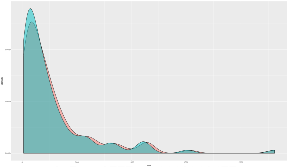
If we compare conditional loss distributions under different dependence assumptions, it shows that the predicted loss with Copula regression tends to have a fatter right tail and therefore should be considered more conservative.

df <- data.frame(g = G, p = P, x1 = X[, 2], x2 = X[, 3])
glm_p <- glm(p ~ x1 + x2, data = df, family = poisson(log))
glm_g <- glm(g ~ x1 + x2, data = df, family = Gamma(log))
loss_dep <- predict(m, X, X, independence = FALSE)[3][[1]][[1]]
loss_ind <- fitted(glm_p) * fitted(glm_g)
den <- data.frame(loss = c(loss_dep, loss_ind), lines = rep(c("DEPENDENCE", "INDEPENDENCE"), each = n))
ggplot(den, aes(x = loss, fill = lines)) + geom_density(alpha = 0.5)