Switzerland’s time series in one place

Similarly to the United States, public data in Switzerland is produced by a large number of different offices, which makes it hard to find any particular series. dataseries.org provides a structured and automatically updated collection of most of these series. We are still working on the data input, but are pretty much complete in the field of Economics.

You can download the data as spreadsheets or graphs, or embed interactive widgets in your website. Alternatively, you can import the data directly into R, using the dataseries package. Install the package from CRAN,

install.packages("dataseries")

and run the ds function with the id argument that you find on the website:

plot(dataseries::ds("GDP.PBRTT.A.R", "ts"), 
     ylab = "mio CHF, at 2010 prices, s. adj.", 
     main = "Gross Domestic Product")

This will give you an R plot of Switzerland’s GDP. (The data is cached, so calling the function again will not re-download until you restart the R session.)

Live Import of Series to R

In the following, I will use data from dataseries.org to produce a live forecast of Switzerland’s GDP. Each day the model is run, it will be ensured that the latest data is used. That way it is possible to produce a transparent and up-to-date forecast. For the following exercise, I will only use tools from R base, but it is of course possible to use the same data in a more advanced modeling framework.

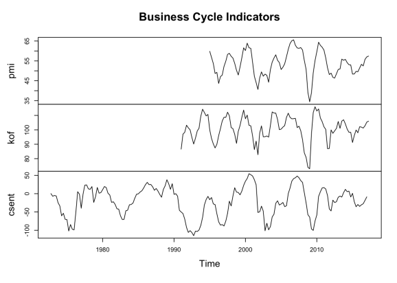
In order to produce a reasonable forecast, we want to track early information on the business cycle, which is mostly survey data. We will use a question from the SECO Consumer Confidence Survey on current economic performance, the Credit Suisse / Procure Purchasing Managers’ Index and the ETHZ KOF Barometer.

Transforming the data

Getting these indicators from dataseries.org directly into R is easy. Because these data are measured at different frequencies, we need to convert them to the same quarterly frequency as GDP. There are many packages that offer functions for that (e.g., the tempdisagg package has functions to move both to higher or lower frequencies), but I will stick to basic R here:

# Aggregating months to quarters
to_quarterly <- function(x){
  sq <- seq(floor(min(time(x))), ceiling(max(time(x))), by = 0.25)
  new.time <- sq[findInterval(time(x), sq)]
  ts(tapply(x, new.time, FUN = mean), start = new.time[1], 
     frequency = 4)
}

pmi <- to_quarterly(dataseries::ds("PMI.SA.PM", "ts"))
kof <- to_quarterly(dataseries::ds("KOF.KFBR", "ts"))
csent <- dataseries::ds("CCI.GEPC", "ts")

A plot of these series shows the common trend in these variables and gives you an indication of the business cycle, which may have turned upward in recent months.

plot(cbind(pmi, kof, csent), main = "Business Cycle Indicators")

Since these series are stationary, our left hand side variable should be stationary as well. This is accomplished by calculating percentage change rates of GDP:

gdp.level <- dataseries::ds("GDP.PBRTT.A.R", "ts")
gdp <- (gdp.level / lag(gdp.level, -1)) - 1

ARIMA modelling

R’s workhorse for time series modeling is the arima function, which allows you to construct a univariate or multivariate model of GDP growth. Since the data is seasonally adjusted, a simple autoregressive process (AR1) offers a good benchmark:

# AR1
m0 <- arima(gdp, order = c(1, 0, 0))
fct0 <- predict(m0, n.ahead = 1)$pred
# GDP Growth Q1: +0.3 

If you need advice on which ARIMA model to choose, the information criterions, accessed by the R functions AIC or BIC, can help you to choose a model. Simply take the model with lowest information criterion. The auto.arima function from the forecast package also allows you to do the selection automatically.

We can include our series individually or jointly and estimate a range of different models. A good model (in terms of the AIC information criterion) is the following, which uses PMI and KOF data (but not consumer sentiment data):

# PMI, KOF
dta <- window(cbind(pmi, kof), start = start(pmi), end = end(pmi))
m1 <- arima(window(gdp, start = start(dta)), 
            xreg = window(dta, end = end(gdp)))
fct1 <- predict(m1, n.ahead = 1, 
                newxreg = window(dta, start = tsp(gdp)[2] + 0.25,
                                 end = tsp(gdp)[2] + 0.25)
                )$pred
# GDP Growth Q1: +0.7

The model’s forecast for the first quarter of 2017 is 0.7 – a value that hasn’t been reached for more than two years.

A factor model

If you have multiple indicators at hand, a common problem is multicollinearity, the fact that indicators are correlated, and therefore too many indicators deteriorate the quality of the model estimation.

An easy fix is to use a factor model, where the indicators are summarized in a few factors, which can be calculated by principal components (see Stock and Watson 2002):

# PMI, KOF, Consumer Sentiment, first Principal Component
pca <- prcomp(window(cbind(pmi, kof, csent), start = start(pmi), 
                     end = tsp(gdp)[2] + 0.25),
             scale. = TRUE)
dta.pca <- ts(pca$x[, 'PC1'], start = start(pmi), frequency = 4)

m2 <- arima(window(gdp, start = start(dta)), 
            xreg = window(dta.pca, end = end(gdp)))
fct2 <- predict(m2, n.ahead = 1, 
                newxreg = window(dta.pca, start = tsp(gdp)[2] + 0.25)
                )$pred
# GDP Growth Q1: +0.7

Again, we get a forecast value of 0.7. Overall, survey data indicates that the economy is well on track. Let’s do a graphical comparison of our forecasts:

# skeletons to include forecasts 
gdp.fct0 <- window(gdp, extend = TRUE, end = tsp(gdp)[2] + 0.25)
gdp.fct1 <- gdp.fct2 <- gdp.fct0

# plug forecasts into skeletons
window(gdp.fct0, start = end(gdp.fct0)) <- fct0
window(gdp.fct1, start = end(gdp.fct1)) <- fct1
window(gdp.fct2, start = end(gdp.fct2)) <- fct2

ts.plot(window(cbind(gdp, gdp.fct0, gdp.fct1, gdp.fct2), 
               start = 2010), 
        col = 1:4, ylab = "quarterly growth rates, s. adj.", 
        main = "GDP Forecasts")
legend("topright", legend = c("GDP Growth Rate", "AR 1 Forecast", 
                              "PMI, KOF", "Principal Component"), 
       lty = 1, col = 1:4, bty = "n")

Publication of first quarter GDP is on June 1, 2017. See you in a month!