Ben Goodrich writes:

The rstanarm R package, which has been mentioned several times on stan-users, is now available in binary form on CRAN mirrors (unless you are using an old version of R and / or an old version of OSX). It is an R package that comes with a few precompiled Stan models — which are called by R wrapper functions that have the same syntax as popular model-fitting functions in R such as glm() — and some supporting R functions for working with posterior predictive distributions. The files in its demo/ subdirectory, which can be called via the demo() function, show how you can fit essentially all of the models in Gelman and Hill’s textbook

http://stat.columbia.edu/~gelman/arm/

and rstanarm already offers more (although not strictly a superset of the) functionality in the arm R package.

The rstanarm package can be installed in the usual way with

install.packages(“rstanarm”)

which does not technically require the computer to have a C++ compiler if you on Windows / Mac (unless you want to build it from source, which might provide a slight boost to the execution speed). The vignettes explain in detail how to use each of the model fitting functions in rstanarm. However, the vignettes on the CRAN website

https://cran.r-project.org/web/packages/rstanarm/index.html

do not currently show the generated images, so call browseVignettes(“rstanarm”). The help(“rstarnarm-package”) and help(“priors”) pages are also essential for understanding what rstanarm does and how it works. Briefly, there are several model-fitting functions:

• stan_lm() and stan_aov(), which just calls stan_lm(), use the same likelihood as lm() and aov() respectively but add regularizing priors on the coefficients
• stan_polr() uses the same likelihood as MASS::polr() and adds regularizing priors on the coefficients and, indirectly, on the cutpoints. The stan_polr() function can also handle binary outcomes and can do scobit likelihoods.
• stan_glm() and stan_glm.nb() use the same likelihood(s) as glm() and MASS::glm.nb() and respectively provide a few options for priors
• stan_lmer(), stan_glmer(), stan_glmer.nb() and stan_gamm4() use the same likelihoods as lme4::lmer(), lme4::glmer(), lme4::glmer.nb(), and gamm4::gamm4() respectively and basically call stan_glm() but add regularizing priors on the covariance matrices that comprise the blocks of the block-diagonal covariance matrix of the group-specific parameters. The stan_[g]lmer() functions accept all the same formulas as lme4::[g]lmer() — and indeed use lme4’s formula parser — and stan_gamm4() accepts all the same formulas as gamm::gamm4(), which can / should include smooth additive terms such as splines

If the objective is merely to obtain and interpret results and one of the model-fitting functions in rstanarm is adequate for your needs, then you should almost always use it. The Stan programs in the rstanarm package are better tested, have incorporated a lot of tricks and reparameterizations to be numerically stable, and have more options than what most Stan users would implement on their own. Also, all the model-fitting functions in rstanarm are integrated with posterior_predict(), pp_check(), and loo(), which are somewhat tedious to implement on your own. Conversely, if you want to learn how to write Stan programs, there is no substitute for practice, but the Stan programs in rstanarm are not particularly well-suited for a beginner to learn from because of all their tricks / reparameterizations / options.

Feel free to file bugs and feature requests at

https://github.com/stan-dev/rstanarm/issues

If you would like to make a pull request to add a model-fitting function to rstanarm, there is a pretty well-established path in the code for how to do that but it is spread out over a bunch of different files. It is probably easier to contribute to rstanarm, but some developers may be interested in distributing their own CRAN packages that come with precompiled Stan programs that are focused on something besides applied regression modeling in the social sciences. The Makefile and cleanup scripts in the rstanarm package show how this can be accomplished (which took weeks to figure out), but it is easiest to get started by calling rstan::rstan_package_skeleton(), which sets up the package structure and copies some stuff from the rstanarm GitHub repository.

On behalf of Jonah who wrote half the code in rstanarm and the rest of the Stan Development Team who wrote the math library and estimation algorithms used by rstanarm, we hope rstanarm is useful to you.

Also, Leon Shernoff pointed us to this post by Wayne Folta, delightfully titled “R Users Will Now Inevitably Become Bayesians,” introducing two new R packages for fitting Stan models:  rstanarm and brms.  Here’s Folta:

There are several reasons why everyone isn’t using Bayesian methods for regression modeling. One reason is that Bayesian modeling requires more thought . . . A second reason is that MCMC sampling . . . can be slow compared to closed-form or MLE procedures. A third reason is that existing Bayesian solutions have either been highly-specialized (and thus inflexible), or have required knowing how to use a generalized tool like BUGS, JAGS, or Stan. This third reason has recently been shattered in the R world by not one but two packages: brms and rstanarm. Interestingly, both of these packages are elegant front ends to Stan, via rstan and shinystan. . . . You can install both packages from CRAN . . .

He illustrates with an example:

Note the more sparse output, which Gelman promotes. You can get more detail with summary (br), and you can also use shinystan to look at most everything that a Bayesian regression can give you. We can look at the values and CIs of the coefficients with plot (mm), and we can compare posterior sample distributions with the actual distribution with: pp_check (mm, "dist", nreps=30):

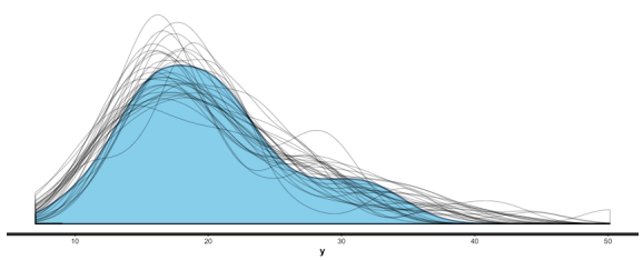
This is all great.  I’m looking forward to never having to use lm, glm, etc. again.  I like being able to put in priors (or, if desired, no priors) as a matter of course, to switch between mle/penalized mle and full Bayes at will, to get simulation-based uncertainty intervals for any quantities of interest, and to be able to build out my models as needed.

The post rstanarm and more! appeared first on Statistical Modeling, Causal Inference, and Social Science.