
A Practical Example of Calculating Padé Approximant Coefficients Using R
Want to share your content on R-bloggers? click here if you have a blog, or here if you don't.
Introduction
I recently had the opportunity to use Padé approximants. There is a lot of good information available on line on the theory and applications of using Padé approximants, but I had trouble finding a good example explaining just how to calculate the co-efficients.
Basic Background
Hearken back to undergraduate calculus for a moment. For a given function, its The Taylor series is the “best” polynomial representations of that function. If the function is being evaluated at 0, the Taylor series representation is also called the Maclaurin series. The error is proportional to the first “left-off” term. Also, the series is only a good estimate in a small radius around the point for which it is calculated (e.g. 0 for a Maclaurin series).
Padé approximants estimate functions as the quotient of two polynomials. Specifically, given a Taylor series expansion of a function  of order
  , there are two polynomials,
  of order
  and
and  of order
  , such that
  , called the Padé approximant of order
 ![[m/n]](https://i2.wp.com/www.avrahamadler.com/wp-content/ql-cache/quicklatex.com-fd327203e6450bd1b185ead8819b0f69_l3.png?resize=42%2C18 "Rendered by QuickLaTeX.com") , “agrees” with the original function in order . You may ask, “but the Taylor series from whence it is derived is also of order ?” And you would be correct. However, the Padé approximant seems to consistently have a wider radius of convergence than its parent Taylor series, and, being a quotient, is composed of lower-degree polynomials. With the normalization that the first term of is always 1, there is a set of linear equations which will generate the unique Padé approximant coefficients. Letting
, “agrees” with the original function in order . You may ask, “but the Taylor series from whence it is derived is also of order ?” And you would be correct. However, the Padé approximant seems to consistently have a wider radius of convergence than its parent Taylor series, and, being a quotient, is composed of lower-degree polynomials. With the normalization that the first term of is always 1, there is a set of linear equations which will generate the unique Padé approximant coefficients. Letting  be the coefficients for the Taylor series, one can solve:
(1) 
remembering that all  m” title=”Rendered by QuickLaTeX.com” height=”17″ width=”75″ style=”vertical-align: -4px;”/> and
  n” title=”Rendered by QuickLaTeX.com” height=”17″ width=”69″ style=”vertical-align: -4px;”/> are 0.
There is a lot of research on the theory of Padé approximants and Padé tables, how they work, their relationship to continued fractions, and why they work so well. For example, the interested reader is directed to Baker (1975), Van Assche (2006), Wikipedia, and MathWorld for more.
Practical Example
The function  will be used as the example. This function has a special representation in almost all computer languages, often called
 log1p(x), as naïve implementation as log(1 + x) will suffer catastrophic floating point errors for  near 0.
The Maclaurin series expansion for is:
![\[ \sum_{k=1}^\infty -1^{k+1}\frac {x^k}{k} = x - \frac{1}{2}x^2 + \frac{1}{3}x^3 - \frac{1}{4}x^4 + \frac{1}{5}x^5 - \frac{1}{6}x^6\ldots \]](https://i2.wp.com/www.avrahamadler.com/wp-content/ql-cache/quicklatex.com-3f0dfbeb2756d35a2e1fd08e28116319_l3.png?resize=417%2C51 "Rendered by QuickLaTeX.com")
The code below will compare a Padé[3,3] approximant with the 6-term Maclaurin series, which would actually be the Padé[6/0] approximant. First to calculate the coefficients. We know the Maclaurin coefficients, they are  . Therefore, the system of linear equations looks like this:
(2) 
Rewriting in terms of the known coefficients, we get:
(3) 
We can solve this in R using solve:
A <- matrix(c(0, 0, 1, -.5 ,1 / 3 , -.25, .2, 0, 0, 0, 1, -.5, 1 / 3, -.25, 0, 0, 0, 0, 1, -.5, 1 / 3, -1, 0, 0, 0, 0, 0, 0, 0, -1, 0, 0, 0, 0, 0, 0, 0, -1, 0, 0, 0, 0, 0, 0, 0, -1, 0, 0, 0), ncol = 7)
B <- c(0, -1, .5, -1/3, .25, -.2, 1/6)
P_Coeff <- solve(A, B)
print(P_Coeff)
## [1] 1.5000000 0.6000000 0.0500000 0.0000000 1.0000000 1.0000000 0.1833333
Now we can create the estimating functions:
ML <- function(x){x - .5 * x ^ 2 + x ^ 3 / 3 - .25 * x ^ 4 + .2 * x ^ 5 - x ^ 6 / 6}

PD33 <- function(x){
  NUMER <- x + x ^ 2 + 0.1833333333333333 * x ^ 3
  DENOM <- 1 + 1.5 * x + .6 * x ^ 2 + 0.05 * x ^ 3
  return(NUMER / DENOM)
}
Let’s compare the behavior of these functions around 0 with the naïve and sophisticated implementations of
 in R.
in R.library(dplyr) library(ggplot2) library(tidyr) D <- seq(-1e-2, 1e-2, 1e-6) RelErr <- tbl_df(data.frame(X = D, Naive = (log(1 + D) - log1p(D)) / log1p(D), MacL = (ML(D) - log1p(D)) / log1p(D), Pade = (PD33(D) - log1p(D)) / log1p(D))) RelErr2 <- gather(RelErr, Type, Error, -X) RelErr2 %>% group_by(Type) %>% summarize(MeanError = mean(Error, na.rm = TRUE)) %>% knitr::kable(digits = 18)
| Type | MeanError |
|---|---|
| Naïve | -4.3280e-15 |
| MacL | -2.0417e-14 |
| Pade | -5.2000e-17 |
Graphing the relative error in a small area around 0 shows the differing behaviors. First, against the naïve implementation, both estimates do much better.
ggplot(RelErr2, aes(x = X)) + geom_point(aes(y = Error, colour = Type), alpha = 0.5)

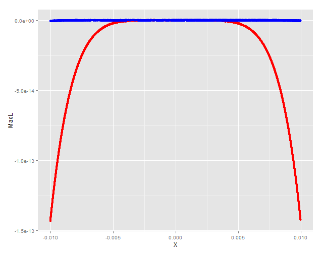
But when compared one against the other, the Pade approximant (blue) shows better behavior than the Maclaurin (red) and it’s relative error stays below EPS for a wider swath.
ggplot(RelErr, aes(x = X)) + geom_point(aes(y = MacL), colour = 'red', alpha = 0.5) + geom_point(aes(y = Pade), colour = 'blue', alpha = 0.5)
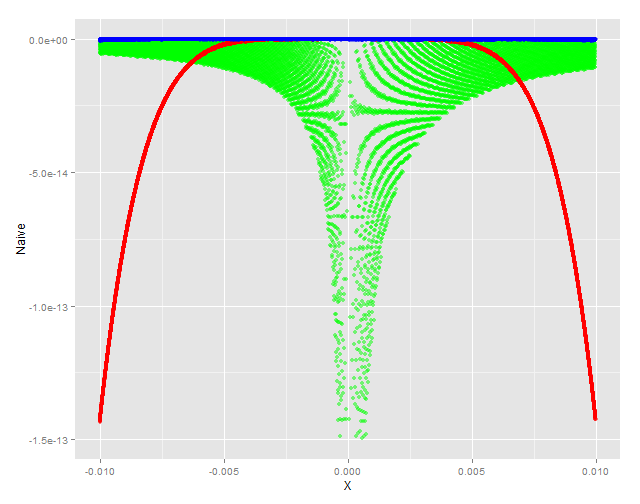
Just for fun, restricting the y axis to that above, overlaying the naïve formulation (green) looks like this:
ggplot(RelErr, aes(x = X)) + geom_point(aes(y = Naive), colour = 'green', alpha = 0.5) + scale_y_continuous(limits = c(-1.5e-13, 0)) + geom_point(aes(y = MacL), colour = 'red', alpha = 0.5) + geom_point(aes(y = Pade), colour = 'blue', alpha = 0.5)
There are certainly more efficient and elegant ways to calculate Padé approximants, but I found this exercise helpful, and I hope you do as well!
References
- Baker, G. A. Essentials of Padé Approximants Academic Press, 1975
- Van Assche, W. Pade and Hermite-Pade approximation and orthogonality ArXiv Mathematics e-prints, 2006
R-bloggers.com offers daily e-mail updates about R news and tutorials about learning R and many other topics. Click here if you're looking to post or find an R/data-science job.
Want to share your content on R-bloggers? click here if you have a blog, or here if you don't.