I just finished covering a few numerical techniques for solving systems of equations, which can be applied to find best-fit lines through a give set of data points.

The four points  are arranged into an inconsistent system of four equations and two unknowns:

The system can be represented in matrix form:

The least-squares solution vector can be found by solving the normal equations

Solving for and yields the following matrix system:

The system can be solved using Gauss-Seidel method.

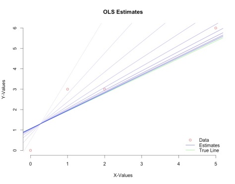
Below, I run 10 iterations of Gauss-Seidel (visualized in the figure above). The estimated line gets successively closer to the true solution in green. The estimates are shown in blue – each iteration is shown in a darker shade than the next (see highlighted lines).

library(MASS) # package needed for ginv() function 

A=cbind(c(4,8),c(8,30)) # coefficient matrix
b<-t(t(c(12,39))) # b-vector
x0<-t(t(c(0,0)))  # starting vector
iter<-10          # number of Gauss-Seidel iterations to run

L<-lower.tri(A)*A  # lower triang. A
U<-upper.tri(A)*A  # upper triang. A
D<-diag(diag(A))   # diag of A

# plot points 
xc<-c(0,1,2,5)
yc<-c(0,3,3,6)
plot(xc,yc,
     col='red',
     xlab="X-Values",
     ylab="Y-Values",
     bty='n')
title(main="OLS Estimates")
legend("bottomright",
       c("Data","Estimates","True Line"),
       lty=c(0,1,1),
       pch=c(1,NA,NA),
       col=c("red","blue","green"),
       bty='n')

# create color palette - lines will get darker with each iter
pal<-colorRampPalette(c("#f2f2f2", "Blue"))
colors<-pal(iter) # creates color palette of length(iter)

# plot true line
abline(a=1.0714,b=.8571,col='green')

n<-1
while(n<=iter){
  print(x0)
  
  # Gauss-Seidel formula
  x1<-(ginv((L+D)))%*%((-U%*%x0)+b)
  x0<-x1
  n=n+1
  
  # plot estimated line  
  abline(a=as.numeric(x0[2,1]), # slope of estimated line
         b=as.numeric(x0[1,1]), # y-intercept of estimated line
         col=colors[n]) # pick nth color in palette
}