A week ago, I wrote a bit about my personal journey to come to grips with Bayesian inference. I referred to the epiphany that when we're talking about Bayesian analysis, what we're talking about- in a tangible way- is using and modifying multivariate distributions. This reminds me of the moment, about twenty years ago now, when I had a nascent interest in object oriented programming. I had read about it, worked through some tutorials and struggled to write any code of my own. I spent a bit of time with a fantastic programmer that I knew, who showed me some code that he and a team of developers were putting together. This was commercial grade software, meant for delivery to clients who would be paying real money for it. And it was straightforward. I said, “John, this really doesn't seem all that strange. It looks like the same code that I'm currently writing.” John responded with a very patient nod of his head. Sure there were some subtle, yet meaningful differences, but I got over my mental hurdle and have been an OOP fan ever since. (No one would mistake me for an expert. I'm a fan.) I'm hoping that Bayes will work out the same and I think that dealing with the multivariate mechanics is the way forward. The math is just too simple.

OK, that last comment may have been a bit much. The math isn't always simple and heaven knows, I'm lost with anything more than two variables. My last post dealt with the simplest multivariate distribution possible- a 2 dimensional Bernouli trial. Now I'm going to do something a bit more complicated. I'm not going to use more than two variables- I doubt my head could take it- but I will at least move to a continuous distribution. My favorite probability distributions are the binomial (only two things to think about!) and the Pareto (discrete! nothing negative!). The only continuous distribution for which I have any fondness is the exponential (one parameter!). It's simple and I like the “lack of memory” property. As an aging drinker, I can identify with that. Moreover, if you combine more than one, you can create a semiparametric model which can support all kinds of curves. So, an exponential distribution it is.

This won't resemble any real-world phenomeon that I can think of. If you need to assume something, you can think of time until a customer service representative answers your call. And, let's say you're calling to trying to make changes to an airlines reservation. US residents may assume American Airlines and feel free to expect that the time may be eternal and with an unhappy resolution. Residents in other countries may substitute Lufthansa, RyanAir, Aeroflot or something similar. (Actually, Lufthansa was always fantastic if travel plans didn't need to be altered. Great planes, great staff. But changing a booking was often a Kafka-esque experience)

So, because this is Bayesian we need another parameter. I'll use the lognormal because it's simple and has support across the set of positive numbers. To simplify, I'm going to presume that I know the variance. (Aside: virtually every beginning stats book that I've read contains exercises where the variance is know, but the mean is not. This has always seemed crazy to me. I can't imagine a circumstance where I emphatically know how much observations vary around the mean, but I don't know the mean itself. The only thing crazier is an obsession with urns. A survey of the work of John Keats would have fewer uses of the word “urn.”)

Right. Back to the math. I'm going to use a lognormal with a mean of 5 and a CV of 20%. Let's draw a quick picture.

mean = 5
cv = 0.2
sigma = sqrt(log(1 + cv^2))
mu = log(mean) - sigma^2/2

plotLength = 100
theta = seq(0.001, 10, length = plotLength)
y = dlnorm(theta, mu, sigma)
plot(theta, y, type = "l")

And now an exponential. Note that for the parameter, I'll be discussing it in such a way that the expected value is equal to the parameter. I think that often, the parameter is set so that the expected value is equal to the reciprocal of the parameter. Actuaries learned it differently- or at least this one did. I don't have my copy of Loss Models with me (it's at work, where it might do me some good), but that's how I'm used to thinking about it.

So, knowing that the exponential parameter could be any positive real number- but expecting it to be something close to 5- let's draw some exponential curves. We’ll use tau as the parameter for waiting time.

tau = seq(0.001, 20, length = plotLength)
t1 = dexp(tau, 1)
t2 = dexp(tau, 1/2)
t3 = dexp(tau, 1/5)
t4 = dexp(tau, 1/10)
plot(tau, t1, type = "l")
lines(tau, t2)
lines(tau, t3)
lines(tau, t4)

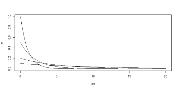
Not terribly pretty, but that's the exponential. No mode, most of the probability shoved to the left hand side, the higher mean distributions wholly reliant on remote, but high valued occurrences.

Now I'm going to render this in two-dimensional space.

dfJoint = expand.grid(Theta = theta, Tau = seq(0.001, 10, length = plotLength))

dfJoint$LogProb = dlnorm(dfJoint$Theta, mu, sigma)
dfJoint$ExpProb = dexp(dfJoint$Tau, 1/dfJoint$Theta)
dfJoint$JointProb = with(dfJoint, LogProb * ExpProb)
dfJoint$JointProb = dfJoint$JointProb/sum(dfJoint$JointProb)

jointProb = matrix(dfJoint$JointProb, plotLength, plotLength)

filled.contour(x = unique(dfJoint$Theta), y = unique(dfJoint$Tau), z = jointProb, 
    color.palette = heat.colors, xlab = "Theta", ylab = "Tau")

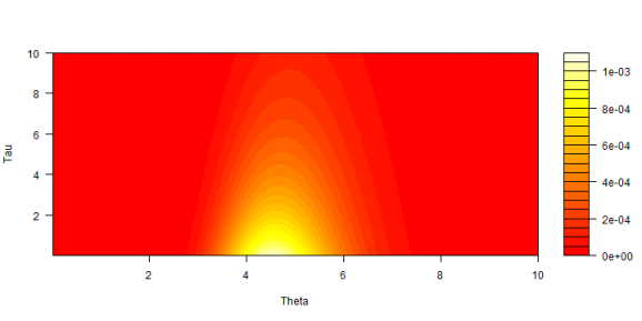
Most of the probability is for tau less than 4 and theta around 5. Each change in color looks a bit like a lognormal distribution as it should. The shift from one lognormal to another follows an exponential curve. Rapid near the bottom, then slower away going towards the top.

As with the cancer example, all of the probability is here. What is the chance that I'll be on hold for longer than 5 minutes? That can be obtained using the marginal exponential distribution. I'm going to cheat and calcuate the marginal based on the subset of the probability space that I used to create the plot.

library(plyr)
marginalExp = ddply(dfJoint[, c("Tau", "JointProb")], .variables = "Tau", summarize, 
    marginalProb = sum(JointProb))
sum(marginalExp$marginalProb[marginalExp$Tau > 5])

## [1] 0.2588

plot(marginalExp$Tau, marginalExp$marginalProb, type = "l", xlab = "Tau", ylab = "Marginal probability")

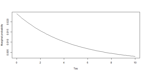
About a 1 in 4 chance. American Airlines should be so lucky. Still, though, this is promising. What I'm most interested in is making predictions and the marginal allows me to do that. I reached this marginal by assuming a prior density- both form and parameters- for another distribution which controls my undestanding of a random event. This is an additional step. Ordinarily, I just work with the one function. Does the addition of another clarify or obscure things? My immediate reaction is to say yes, because- ceteris paribus- more information is preferred over less information. I hope to explore this in my next post, where I'll try to use some real-world example. Suggestions welcome.

Session info:

## R version 3.0.2 (2013-09-25)
## Platform: x86_64-w64-mingw32/x64 (64-bit)
## 
## locale:
## [1] LC_COLLATE=English_United States.1252 
## [2] LC_CTYPE=English_United States.1252   
## [3] LC_MONETARY=English_United States.1252
## [4] LC_NUMERIC=C                          
## [5] LC_TIME=English_United States.1252    
## 
## attached base packages:
## [1] stats     graphics  grDevices utils     datasets  methods   base     
## 
## other attached packages:
## [1] knitr_1.5        RWordPress_0.2-3 plyr_1.8        
## 
## loaded via a namespace (and not attached):
## [1] evaluate_0.5.1 formatR_0.10   RCurl_1.95-4.1 stringr_0.6.2 
## [5] tools_3.0.2    XML_3.98-1.1   XMLRPC_0.3-0