
24 Days of R: Day 15
Over the course of the next few days, I'm going to try to find enough time to build up a reasonably simple simulation of insurance exposure and claims. I'll be taking a hierarchical view of the underlying process. As with pretty much everything that I write about, I'm writing about it as I'm learning about it. It was only last year that I first started getting familiar with the Andrew Gelman and Jennifer Hill text, which is a fantastic book. Over the time that I've had the book, I've peruse it, but have not yet really gotten my hands dirty with it in practice.
I'm going to look at a claim count generation process where the number of claims is Poisson distributed. The Poisson parameter will be keyed to exposure at a later stage, but for now, we'll assume a constant level of exposure. I'll presume that I'm looking at the business of a national insurance carrier, based in the United States, which experiences claims in all of the 50 states and DC. As a first step, I'll assume a two level hierarchy. There is a “national” distribution of lambda parameters and each state has its own distribution, which is based on a random draw from the national distribution.
Again drawing inspiration from Jim Albert's book Bayesian Computation with R, I'll assume that the national parameter is taken as a random draw from a gamma. An expected value of ten claims per year seems interesting enough. As for the variance, I'd like a 10% chance that lambda is greater than 25. This time, I'll not be lazy and will use the optim function to determine that scale parameter which will give me this distribution. I'm using a slightly ham-fisted objective function wherein I combine two constraints.
fff = function(pars) {
shape = pars[1]
scale = pars[2]
y = abs(25 - qgamma(0.9, shape = shape, scale = scale))
z = abs(10 - shape * scale)
y + z
}
pars = optim(par = list(shape = 10, scale = 2), fff)
## Warning: NaNs produced
scale = pars$par["scale"]
shape = pars$par["shape"]
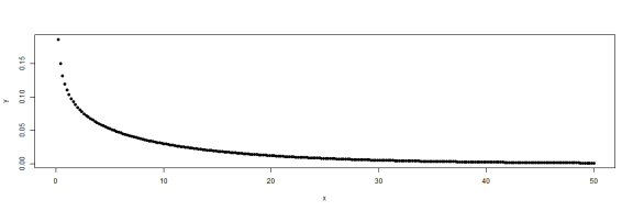
x = seq(from = 0, to = 50, length.out = 250)
y = dgamma(x, shape, scale = scale)
plot(x, y, pch = 19)
# shape * scale qgamma(0.9, shape = shape, scale = scale)
Functions without a mode make me nervous, but I suppose that's the price to pay for this level of variance. Given this function, I'll generate 51 lambdas for the second level of the simulation.
numStates = 51
set.seed(1234)
lambdas = rgamma(numStates, shape = shape, scale = scale)
x = 1:numStates
y = lambdas
plot(x, y, pch = 19)
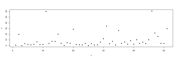
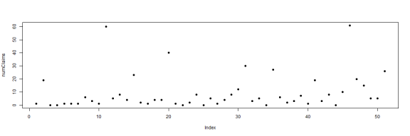
Cool. Loads of variation from 0.0282 to 60.6984. Note that these are just parameters. The actual claims numbers will be random realizations of Poisson distributions. So what sort of claims do we seen in a particular year?
numClaims = rpois(numStates, lambdas)
plot(numClaims, pch = 19)
par(mfrow = c(1, 1))
plot(lambdas, pch = 19, ylim = c(0, 70))
points(numClaims, pch = 19, ylim = 70, col = "red")
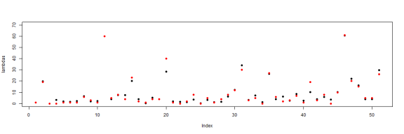
Very close to the expectation. The interesting thing is that if I were to look at these claims, I would assume that most came from different distributions. Particularly the states which produce large lambdas. It would be reasonable to assume that there are loss characteristics which are the result of particular dynamics in that state. But this assumption would be wrong. It's possible to continue this at many finer levels of detail and I'll do so. Tomorrow.
sessionInfo()

## R version 3.0.2 (2013-09-25)
## Platform: x86_64-w64-mingw32/x64 (64-bit)
##
## locale:
## [1] LC_COLLATE=English_United States.1252
## [2] LC_CTYPE=English_United States.1252
## [3] LC_MONETARY=English_United States.1252
## [4] LC_NUMERIC=C
## [5] LC_TIME=English_United States.1252
##
## attached base packages:
## [1] stats     graphics  grDevices utils     datasets  methods   base
##
## other attached packages:
## [1] knitr_1.4.1      RWordPress_0.2-3
##
## loaded via a namespace (and not attached):
## [1] digest_0.6.3   evaluate_0.4.7 formatR_0.9    RCurl_1.95-4.1
## [5] stringr_0.6.2  tools_3.0.2    XML_3.98-1.1   XMLRPC_0.3-0
