
Modified Bin and Union Method for Item Pool Design
[This article was first published on Econometrics by Simulation, and kindly contributed to R-bloggers]. (You can report issue about the content on this page here)
Want to share your content on R-bloggers? click here if you have a blog, or here if you don't.
Want to share your content on R-bloggers? click here if you have a blog, or here if you don't.
# Reckase (2003) proposes a method for designing an item pool for a computer
# adaptive test that has been known as the bin and union method. This method
# involves drawing a subject from a distribution of abilities. Then selecting
# the item that maximizes that subject's information from the possible set of
# all items given a standard CAT proceedure. This is repeated until the test
# reaches the predifined stopping point.
# Then then next subject is drawn and a new set of items is drawn. Items are
# divided into bins such that there is a kind of rounding. Items which are
# sufficiently close to other items it terms of parameter fit are considered
# the same item and the two sets are unionized together into a larger pool.
# As more subjects are added more items are collected though at a decreasing
# rate as fewer new items become neccessary.
# In the original paper he uses a fixed length test though in a forthcoming
# paper he and his student Wei He is also using a variable length test.
# I have modified his proceedure slightly in this simulation. Rather than
# selecting optimal items for each subject based from the continuous pool
# of possible items I have the test look within the already constructed pool
# to see if any items are within bin length of the subject's estimated ability.
# If there is no item then I add an item that perfectly matches the subject's
# estimated ability. The reason I prefer this method is that I think it better
# represents the process that a CAT test typically must go through with items
# close to but rarely exactly at the level of the subjects. Thus the information
# for each subject will be slightly less as a result of this modified method
# relative to the original.
# As with the new paper this simulation uses a variable length test. My stopping
# rule is simple. Once the test achieves a sufficiently high level of
# information, then it stops.
# I have constructed this simulation as one with three nested loops.
# Over subjects within the item pool construction.
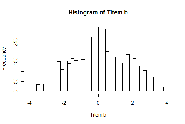
# It simulates the item pool construction a number of times to get the
# average number of items after each subject as well as a histogram
# of average number of items required at each difficulty level.
# I have also included a control for item exposure. This control
# dicatates that as the acceptable exposure rate is reduced, more items
# will be required since some are too frequently exposed.
# Overall this method is seems pretty great to me. It allows for
# item selection criteria, stopping rules, and exposure controls
# to be easily modified to accomidate most any CAT design.
require("catR")
# Variable Length Test
# The number of times to repeat the simulation
nsim <- 10
# The number of subjects to simulate
npop <- 1000
# The maximum number of items
max.items <- 5000
# Maximum exposure rate of individual item
max.exposure <- .2
# Stop the test when information reaches this level
min.information <- 10
# How far away will the program reach for a new item (b-b_ideal)
bin.width <- .25
expect.a <- 1
p <- function(theta, b) exp(theta-b)/(1+exp(theta-b))
info <- function(theta, b, a=expect.a) p(theta,b)*(1-p(theta,b))*a^2
info(0,0)
# The choose.item funciton takes an input thetahat and searches
# available items to see if any already exist that can be used
# otherwise it finds a new item.
choose.item <- function(thetahat, item.b, items.unavailable, bin.width) {
# Construct a vector of indexes of available items
avail.n <- (1:length(item.b))
# Remove any already make unusuable
if (length(items.unavailable)>0)
avail.n <- (1:length(item.b))[-items.unavailable]
# If there are no items available then generate the next item
# equal to thetaest.
if (length(avail.n)==0)
return(c(next.b=thetahat, next.n=length(item.b)+1))
# Figure out how far each item is from thetahat
avail.dist <- abs(item.b[avail.n]-thetahat)
# Reorder the n's and dist in terms of proximity
avail.n <- avail.n[order(avail.dist)]
avail.dist <- sort(avail.dist)
# If the closest item is within the bin width return it
if (avail.dist[1]<bin.width)
return(c(next.b=item.b[avail.n[1]], next.n=avail.n[1]))
# Otherwise generate a new item
if (avail.dist[1]>=bin.width)
return(c(next.b=thetahat, next.n=length(item.b)+1))
}
# Define the simulation level vectors which will become matrices
Tnitems <- Ttest.length <- Titems.taken.N <- Titem.b<- NULL
# Loop through the number of simulations
for (j in 1:nsim) {
# Seems to be working well
choose.item(3, c(0,4,2,2,3.3), NULL, .5)
# This is the initial item pool
item.b <- 0
# This is the initial number of items taken
items.taken.N <- rep(0,max.items)
# A vector to record the individual test lengths
test.length <- NULL
# Number of total items after each individual
nitems <- NULL
# Draw theta from a population distribution
theta.pop <- rnorm(npop)
# Start the individual test
for (i in 1:npop) {
# The this person has a theta of:
theta0 <- theta.pop[i]
# Our initial guess at theta = 0
thetahat <- 0
print(paste("Subject:", i,"- Item Pool:", length(item.b)))
response <- items.taken <- NULL
# Remove any items that would have been overexposed
items.unavailable <- (1:length(item.b))[!(items.taken.N < max.exposure*npop)]
# The initial imformation on each subject is zero
infosum <- 0
# Loop through each subject
while(infosum < min.information) {
chooser <- choose.item(thetahat, item.b, items.unavailable, bin.width)
nextitem <- chooser[2]
nextb <- chooser[1]
names(nextitem) <- names(nextb) <- NULL
items.unavailable <- c(items.unavailable,nextitem)
item.b[nextitem] <- nextb
response <- c(response, runif(1)<p(theta0, nextb))
items.taken <- c(items.taken, nextitem)
it <- cbind(1, item.b[items.taken], 0,1)
thetahat <- thetaEst(it, response)
infosum <- infosum+info(theta0, nextb)
}
# Save individual values
nitems <- c(nitems, length(item.b))
test.length <- c(test.length, length(response))
items.taken.N[items.taken] <- items.taken.N[items.taken]+1
}
# Save into matrices the results of each simulation
Titem.b <- c(Titem.b, sort(item.b))
Tnitems <- cbind(Tnitems, nitems)
Ttest.length <- cbind(Ttest.length, test.length)
Titems.taken.N <- cbind(Titems.taken.N, items.taken.N)
}
plot(apply(Tnitems, 1, max), type="n",
xlab = "N subjects", ylab = "N items",
main = paste(nsim, "Different Simulations"))
for (i in 1:nsim) lines(Tnitems[,i], col=grey(.3+.6*i/nsim))

# We can see that the number of items is a function of the number of
# subjects taking the exam.  This relationship becomes relaxed
# when the number of subjects becomes large and the exposure controls
# are removed.
hist(Titem.b, breaks=30)
hist(Ttest.length, breaks=20)

To leave a comment for the author, please follow the link and comment on their blog: Econometrics by Simulation.
R-bloggers.com offers daily e-mail updates about R news and tutorials about learning R and many other topics. Click here if you're looking to post or find an R/data-science job.
Want to share your content on R-bloggers? click here if you have a blog, or here if you don't.