
shinyPsychometric: simulating how experimental choices affect results uncertainty
Want to share your content on R-bloggers? click here if you have a blog, or here if you don't.
In the R community, Shiny is trending a lot. Shiny is an R package for developing interactive web applications. I wanted to give it a try, and ended up with an app to simulate the impact of data collection choices on the outcome reliability of a curve fitting process.
I wrote the code behind it for a Master class on research methods in Psychology. During this year-long class, students learn about research by practicing it under the supervision of a staff member. This was the first time they had to design and run a real experiment. I wrote the code to help them make informed choices. Indeed, subtle design choices (e.g. the number of items presented to a participant) may dramatically change the reliability of the results. The app is there to let them experiment before collecting their experimental data.
Experimental data may be far less rock solid that they appear, and this is not obvious to most people. Even more importantly from an educational perspective, the app illustrates the need to quantify/display results uncertainty (see e.g. a paper by Vivien Marx in this year Nature Methods1).
The app
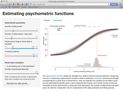
The app running in a browser. Click on the image to start it
The app uses the psychometric function as an example of curve fitting and parameter estimation.

Gustav Theodor Fechner (1801–1887), founder of the psychophysics
The psychometric function relates the strength of an external stimulus and the observer’s responses. Measuring it is a classical method in psychophysics since the mid 19th century and Gustav Fechner.
A standard way to measure one’s psychometric function is to collect an observer’s responses to a number of predetermined stimulus intensities (aka the method of constant stimuli). As an example, a small light dot can be displayed at various light intensities on a steady dark background, and the observer is asked to report the dot presence. The various light intensities are chosen in order to go from ‘not visible at all’ to ‘detectable most of the time’. The order of presentation is randomized, and each level is repeated many times. The observer’s responses (in our example, the probability of detecting the light) are plotted against the stimulus strengths (the light intensity, or contrast), and a sigmoid curve is fitted. This curve is the observer’s psychometric function for light/contrast detection. For historical reasons, a threshold is often estimated: it is the stimulus strength corresponding to a given level of performance (e.g. the light contrast at which the dot is detected 75% of the time).
Experimental choices

The app left panel includes most of the standard choices an experimenter faces when planning to measure a psychometric function with the method of constant stimuli.
As in any experiment, one faces choices when planning to measure a psychometric function: the number of tested stimulus intensities, their particular values, the number of times each intensity is presented, etc. Those choices may greatly affect the reliability of the curve parameters and threshold estimates. There is an abundance of methodological articles to guide the researcher (see e.g. the special issue of Perception & Psychophysics on ‘Threshold Estimation’). This app offers a way to directly experiment with design choices by simulation.
Most standard choices are presented in the app left panel. For each parameter, the default values provided are representative of what can be found in the literature. The ‘performance range’ may deserve some explanation. It is the range (in theoretical probability of the participant’s answer, i.e. along the y axis) in which data will be sampled. The program computes the corresponding values on the stimulus intensity x axis, and places n simulated intensities at equal distances within this interval.
The simulation (or the gist of it)
The app runs a simulation. In this section, I’ll give you the gist of it. How it is coded is shown below.
Everything starts with a predefined psychometric function. This is the ‘real’ psychometric function of our simulated participant. It is shown in red on the plot. When running an experiment, this function is obviously not known, and the experimenter aims at estimating it. However, we know it and randomly draw data from it. This way, we can evaluate how close are the values estimated on the simulated data to the ‘real’ ones from the original function.
For this example, I chose a cumulative Gaussian, with mean arbitrarily set to 0 and standard deviation to 1.
So here is the flow:
- the user modifies an experimental parameter, or hits the ‘Generate new data sample’ button. This sets the particular experimental choices for the simulation;
- At each chosen stimulus intensity, the observer’s answers are simulated by randomly sampling from a binomial distribution. It is a discrete probability function of the number of successes in a sequence of n independent trials. The probability of a correct response at each stimulus intensity is given by the ‘real’ known psychometric function;
- A curve is fitted to the data by maximum likelihood. The curve is a cumulative Gaussian with at least two parameters: its mean and standard deviation. A more general description of the psychometric function is presented below, and adds parameters. The estimated curve is displayed in grey on the upper part of the figure. You can compare it to the known function from which data has been sampled ;
- A threshold is estimated. It is simply the stimulus intensity corresponding to a selected performance level, the threshold criterion. The estimated threshold is shown in the lower part of the figure, along with its real value (in red). You can see how close/far they are from each other as you change the experimental parameters or generate a new sample.
Showing variability
One way to have a feeling of how variable are the results is simply to run the simulation multiple times. After having set your virtual experiment, you can click on the ‘Generate new sample’ button a few times, and watch how the fitted curve changes from one sample to another. It is surprising how variable they are, even with a fair amount of items. However, this give you only a hint of the outcome variability.
A better way is to display the distribution of the results of multiple simulation runs. You can do this by increasing the number of generated data sets from 1 up to 500. Note that this may take some time to compute. Now all estimated curves are displayed on the top panel, with the alpha level adjusted to avoid over-plotting. The bottom panel shows a histogram and a kernel density of the resulting distribution of threshold estimates. Remember that all the data sets have been generated under the same conditions, and represent various possible outcomes of the same experiment. You can assess the impact of different data collection scenarios directly from your browser, just as it has been done more quantitatively in various publications.
A classical and highly cited one (Wichmann and Hill, 20012) discusses the importance to estimate a third parameter of the psychometric function: the lapsing rate. In this more general formalization (see below) of the psychometric function, the function is allowed to asymptote at the maximal performance of 

Running the app
The app is available in two versions:
- one that you can directly access in your browser (link here). It runs on a remote R server hosted and powered by Rstudio (It is currently under beta testing);
- one that you run locally on your computer. It requires to have R and some additional packages installed. Installation instructions are listed at the app github repos.
Having a look at the code
in this section, I will highlight some general aspects of the code. You can have a look at the whole code hosted on github, which is fully commented.
A general form of the psychometric function is
 = \gamma + (1 - \gamma - \lambda)F(x;\alpha,\beta)")
where
is a sigmoid function mapping the stimulus intensity
to the range [0;1], typically a cumulative distribution function of a distributional family. In this app, we use a cumulative Gaussian ;
and
are the location parameters of
) and standard deviation (
); and
and
In our R implementation, we use ")
# parameters of the psychometric function used in this simulation
# Rem: in the functions that define the psychometric function, we use exp(beta), instead of beta, to force beta to be non negative in the fitting procedure. so here we define beta as log(beta)
p <- c(0, log(1), 0.01, 0)
names(p) <- c('alpha', 'logbeta', 'lambda', 'gamma')

# psychometric function
# x are the stimulus intensities
# p is a vector of 4 paramaters: alpha, log(beta), lambda and gamma
# REM Note that we use exp(beta) in the function, to make sure that it is always positive.
# Here we use a cumulative Gaussian (pnorm) as sigmoid function.
# the output is a vector of accurate response probabilities
ppsy <- function(x, p) p[4] + (1- p[3] - p[4]) * pnorm(x, p[1], exp(p[2]))
Similar to the way the classical distribution functions are defined in R (e.g. pnorm(), qnorm() and rnorm()), we declared a quantile function qpsy() and a random generation rpsy() for the psychometric function.
# function to convert probabilities from the psychometric function
# to the underlying cummulative distribution.
# Useful to compute a threshold
# prob is the response probability from $\Psi$ (in the range [gamma; 1-lambda])
# the output is a vector of corresponding probabilities on $F$ (in the range [0;1])
probaTrans <- function(prob, lambda, gamma) (prob-gamma) / (1-gamma-lambda)

# Quantile function (inverse of the psychometric function)
# prob is a vector of probabilities
# p is a vector of 4 paramaters: alpha, log(beta), gamma and lambda
# Here we use a cumulative Gaussian (qnorm) as sigmoid function.
# the output is a vector of stimulus intensities
qpsy <- function(prob, p) qnorm(probaTrans(prob, p[3], p[4]), p[1], exp(p[2]))

# random generation from the psychometric function
# We sample random values from a binomial distribution with probabilities given by the ---known--- underlying psychometric function.
# x are the stimulus intensities
# p is a vector of 4 paramaters: alpha, log(beta), gamma and lambda
# nObs is the number of observations for each stimulus level x
rpsy <- function(x, p, nObs)
{
    prob <- ppsy(x, p)
    rbinom(prob, nObs, prob)
}
There are multiple ways to fit a psychometric function in R. We opted for direct (constrained) log likelihood maximization.
# define the likelihood function
# p is the parameters vector, in the order (alpha, log(beta), lambda, gamma)
# df is a 3-column matrix with the stimulus intensities (df[, 1]), and the number of correct and incorrect responses (df[, 2:3])
# opts is a list of options (set by the user of the shiny app)
likelihood <- function(p, df, opts) {

    # do we estimate lambda?
    if (opts$estimateLambda) {
        # if yes, we set gamma (the last parameter) to 0
        psi <- ppsy(df[, 1], c(p, 0))
    } else {
        # we set both gamma and lambda to 0
        psi <- ppsy(df[, 1], c(p, 0, 0))
    }

    # bayesian flat prior
    # implements the constraints put on lambda, according to Wichmann & Hill
    if (opts$estimateLambda && p[3] > 0.06) {
        -log(0)
    } else {
        # compute the log likelihood
        -sum(df[,2]*log(psi) + df[,3]*log(1-psi))
    }
}

# A function to fit the psychometric function
# There are multiple ways to do it. Here we directly maximize the log likelihood. But see e.g. Knoblauch and Maloney (2012) for some R code examples on how to use glm with special link functions.
# df is a 3-column matrix with the stimulus intensities (df[, 1]), and the number of correct and incorrect responses (df[, 2:3])
# opts is a list of options (set by the user of the shiny app)
fitPsy <- function(df, opts)
{
    if(opts$estimateLambda){
        # estimating $\alpha$, $\beta$ and $\lambda$
        optim(c(1, log(3), 0.025), likelihood, df=df, opts=opts,
            control=list(parscale=c(1, 1, 0.001)))
    } else {
        # estimating $\alpha$, $\beta$
        optim(c(1, log(3)), likelihood, df=df, opts=opts)
    }
}
Other ways include
- using
glm()with the binomial error family and standard link (e.g.logitfor a cumulative Gaussian); - using
glm()with custom links from the psyphy package; - a Bayesian inference procedure provided in package PsychoFun;
- etc.
and are described in e.g.
- Knoblauch, K., & Maloney, L. T. (2012). Modeling Psychophysical Data in R. New York: Springer-Verlag. doi:10.1007/978-1-4614-4475-6
- Yssaad-Fesselier, R., & Knoblauch, K. (2006). Modeling psychometric functions in R. Behavior research methods, 38(1), 28–41. doi:10.3758/BF03192747
- Marx, V. (2013). Data visualization: ambiguity as a fellow traveler. Nature methods, 10(7), 613–615. doi:10.1038/nmeth.2530.↩
- Wichmann, F. A., & Hill, N. J. (2001). The psychometric function: I. Fitting, sampling, and goodness of fit. Perception & Psychophysics, 63(8), 1293–1313. doi:10.3758/BF03194544.↩

R-bloggers.com offers daily e-mail updates about R news and tutorials about learning R and many other topics. Click here if you're looking to post or find an R/data-science job.
Want to share your content on R-bloggers? click here if you have a blog, or here if you don't.