Introduction

Continuing my recent series on exploratory data analysis (EDA), this post focuses on the conceptual foundations of empirical cumulative distribution functions (CDFs); in a separate post, I will show how to plot them in R.  (Previous posts in this series include descriptive statistics, box plots, kernel density estimation, and violin plots.)

To give you a sense of what an empirical CDF looks like, here is an example created from 100 randomly generated numbers from the standard normal distribution.  The ecdf() function in R was used to generate this plot; the entire code is provided at the end of this post, but read my next post for more detail on how to generate plots of empirical CDFs in R.

Read to rest of this post to learn what an empirical CDF is and how to produce the above plot!

What is an Empirical Cumulative Distribution Function?

An empirical cumulative distribution function (CDF) is a non-parametric estimator of the underlying CDF of a random variable.  It assigns a probability of to each datum, orders the data from smallest to largest in value, and calculates the sum of the assigned probabilities up to and including each datum.  The result is a step function that increases by at each datum.

The empirical CDF is usually denoted by or , and is defined as

is the indicator function.  It has 2 possible values: 1 if the event inside the brackets occurs, and 0 if not.

at ,

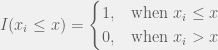
1. count the number of data less than or equal to 
2. divide the number found in Step #1 by the total number of data in the sample

Why is the Empirical Cumulative Distribution Useful in Exploratory Data Analysis?

The empirical CDF is useful because

• it approximates the true CDF well if the sample size (the number of data) is large, and knowing the distribution is helpful for statistical inference
• a plot of the empirical CDF can be visually compared to known CDFs of frequently used distributions to check if the data came from one of those common distributions
• it can visually display “how fast” the CDF increases to 1; plotting key quantiles like the quartiles can be useful to “get a feel” for the data

Some Mathematical Statistics of the Empirical Distribution Function

Some appealing properties of the empirical CDF can be obtained from mathematical statistics.

1) For a fixed , is a Bernoulli random variable with a probability of equalling 1.  Thus, its expected value is

,

which means that is an unbiased estimator of for a fixed .  Also note that its variance is

.

2) By summation of all of these Bernoulli random variables, is a binomial random variable.  Thus,

, so

is also an unbiased estimator of .

Also note that

.

Thus, for a fixed , has a lower variance than .

3) By the Glivenko-Cantelli theorem,  is a consistent estimator of .  In fact, converges uniformly to .

Here is the code for generating the plot of the empirical CDF of the random standard normal numbers; the plot is given again after the code.  For the sake of brevity, I will describe in detail how to generate this and other plots of empirical CDFs in a separate post; in fact, I will show 2 different ways of doing so in R!

##### Empirical Distribution Function
##### By Eric Cai - The Chemical Statistician
# set the seed for consistent replication of random numbers
set.seed(1)

# generate 100 random numbers from the standard normal distribution
normal.numbers = rnorm(100)

# empirical normal CDF of the 100 normal random numbers
normal.ecdf = ecdf(normal.numbers)

# plot normal.ecdf (notice that the only argument needed is normal.ecdf)
# use png() and dev.off() to print this plot to your chosen folder
png('INSERT YOUR DIRECTORY PATH HERE/ecdf standard normal.png')

plot(normal.ecdf, xlab = 'Quantiles of Random Standard Normal Numbers', ylab = '', main = 'Empirical Cumluative Distribution\nStandard Normal Quantiles')

# add label to y-axis with mtext()
# side = 2 denotes the left veritical axis
# line = 2.5 sets the position of the label
mtext(text = expression(hat(F)[n](x)), side = 2, line = 2.5)

dev.off()