In the early days of the discipline of statistics, R.A. Fisher argued with great vehemence against Egon Pearson (and Jerzy Neyman) over the foundational notions supporting statistical inference. The personal invective recorded is somewhat amusing and also reminds us how very puerile even very smart people can be.

Today, we’ll compare Fisher’s exact test for 2*2 tables with the Pearson chi-square, developed by Karl Pearson, Egon’s father and another early pioneer of statistics. This blog entry was inspired by a questioner on LinkedIn who asked when should the one be preferred over the other. One commenter gave the typical rule of thumb– “If the expected count in any cell is less than 5, use the exact test, otherwise use the chi-square.” My copy of “Statistical rules of thumb” is AWOL at the moment, so I don’t know if this one is covered there. A quick googling did not reveal an answer either.

The rule of thumb dates back to the days before the exact test became computationally feasible outside of small problems. In contrast, today it can be performed quickly for all tables, either through a complete enumeration of the possible tables or through Monte Carlo hypothesis testing, which is simple to apply in either SAS or R. My default in recent years has been to take advantage of this capability and use the exact test all the time, ignoring the traditional approximate chi-square test. My idea was that if there were any small cells, I’d be covered, while allowing a simpler methods section.

Let’s develop some code to see what happens. Is the rule of thumb accurate? What’s the power cost of using the exact test instead of the Chi-square?

Our approach will be to set cell probabilities and the sample size, and simulate data under this model, then perform each test and evaluate the proportion of rejections under each test. One complication here is that simulated data might result in a null margin, i.e., there might be no observed values in a row or in a column. We’ll calculate rejections of the null only among the tables where this does not happen. This means that the average observed cell counts among included tables may be different from the expect cell counts. This makes sense from a practical perspective– we probably would not do the test if we observed 0 subjects in one of our planned categories.

SAS
In SAS, we’ll do the dumb straightforward thing and simulate 100 pairs of dichotomous variables. Here we just code the null case of no association, with margins of 70% in one column and 80% in one row. The smallest cell has an expected count of 6%, so that a total sample size of 83 will have an expected count of 5 in that cell.

data test;
pdot1 = .7;
p1dot = .8;
do tablen = 20, 50, 100, 200, 500, 1000;
  do ds = 1 to 10000;
    do i = 1 to tablen;
      xnull = uniform(0) gt pdot1;
      ynull = uniform(0) gt p1dot;
      output;
      end;
    end;
  end;
run;

Then proc freq can be used to generate the two p-values, using the by statement to do the calculations for all the tables at once. The output statement extracts the p-values into a data set.

ods select none;
options nonotes;
proc freq data = test;
by tablen ds;
tables ynull * xnull / chisq fisher;
output out = kk1 chisq fisher;
run;
options notes;
ods select all;

To get the proportion of rejections, we first use a data step to calculate whether each test was rejected, then go back to proc freq to find the proportion of rejections and the CI on the probability of rejections.

data summ;
set kk1 (keep = tablen p_pchi xp2_fish);
rej_pchi = (p_pchi lt 0.05);
rej_fish = (xp2_fish lt .05);
run;

ods output binomialprop = kk2;
proc freq data = summ;
by tablen;
tables rej_pchi rej_fish / binomial(level='1');
run;

You may have noticed that we didn’t do anything to account for the tables with empty rows or columns. When the initial proc freq encounters such a table, it performs neither test. Thus the second proc freq is calculating the proportion and CI with a denominator that might be smaller than the number of tables we simulated. Happily, they’ll still be correct, though the CI may be wider than we’d intended. Finally, we’re ready to plot the results, using the hilob interpolation described in Example 10.4. Using hiloc instead shows the “close” as a tick mark between the high and low values.

data kk2a;
set kk2;
if table eq "Table rej_pchi" then tablen = tablen + 1;
run;

symbol1 i = hiloc;
symbol2 i = hiloc;
proc gplot data = kk2a;
where name1 in ("_BIN_","XL_BIN","XU_BIN");
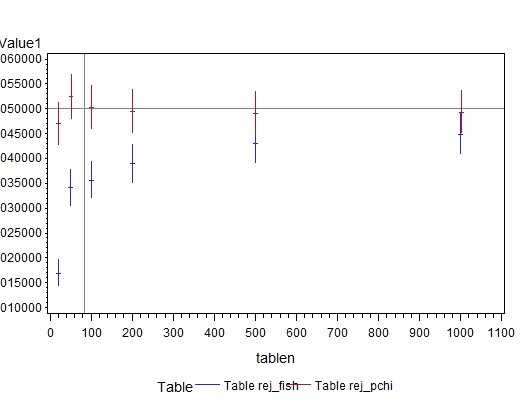
plot nvalue1 * tablen = table / vref = 0.05 href=83;
/* ref lines where the expected count in the smallest cell is > 5, 
and the nominal alpha */
run; quit;

The results are shown above. The confidence limits should include 0.05 for all numbers of subjects in order to be generally recommended. Both tests reach this standard, with these margins, even for tables with only 20 subjects, i.e., with expected cell counts of 11, 5, 3, and 1. The exact test appears conservative (rejects less than 5% of the time), probably due to small cell counts and the resulting ties in the list of possible tables.

R
In R, we’ll simulate observations from a multinomial distribution with the desired cell probabilities, and assemble the result into a table to calculate the p-values. This will make it easier to simulate tables under the alternative, as we need to do to assess power. If there are empty rows or columns, the chisq.test() function produces a p-value of “NaN”, which will create problems later. To avoid this, we’ll put the table generation inside a while() function. This operates like the do while construction in SAS (and other programming languages). The condition we check for is whether there is a row or column with 0 observations; if so, try generating the data again. We begin by initializing the table with 0’s.

makeitm = function(n.in.table, probs)  {
   myt = matrix(rep(0,4), ncol=2)
  while( (min(colSums(myt)) == 0) | (min(rowSums(myt)) == 0) )  { 
    myt = matrix(rmultinom(n=1, size=n.in.table, probs), ncol=2,byrow=TRUE)
}
  chisqp = chisq.test(myt, correct=FALSE)$p.value
  fishp = fisher.test(myt)$p.value
  return(c(chisqp, fishp))
}

With this basic building block in place, we can write a function to call it repeatedly (using the replicate() function, then calculate the proportion of rejections and get the CI for the probability of rejections.

many.ns = function(tablen, nds,probs) {
  res1 = t(replicate(nds,makeitm(tablen,probs)))
  res2 = res1 < 0.05
  pear = sum(res2[,1])/nds
  fish = sum(res2[,2])/nds
  pearci = binom.test(sum(res2[,1]),nds)$conf.int[1:2]
  fishci = binom.test(sum(res2[,2]),nds)$conf.int[1:2]
  return(c("N.ds" = nds, "N.table" = tablen, probs, 
          "Pearson.p" = pear, "PCIl"=pearci[1], "PCIu"=pearci[2],
          "Fisher.p" = fish, "FCIl" = fishci[1], "FCIu" = fishci[2]))
}

Finally, we're ready to actually do the experiment, using sapply() to call the function that calls replicate() to call the function that makes a table. The result is converted to a data frame to make the plotting simpler. The first call below replicates the SAS result shown above and has very similar estimates and CI, but is not displayed here. The second shows an odds ratio of 3, the third (plotted below) has an OR of 1.75, and the last an OR of 1.5.

#res3 = data.frame(t(sapply(c(20, 50, 100, 200, 500, 1000),many.ns, nds=10000, 
  probs = c(.56,.24,.14,.06))))
#res3 = data.frame(t(sapply(c(20, 50, 100, 200, 500, 1000),many.ns, nds=1000, 
  probs = c(.6,.2,.1,.1))))
res3 = data.frame(t(sapply(c(20, 50, 100, 200, 500, 1000),many.ns, nds=1000, 
  probs = c(.58,.22,.12,.08))))
#res3 = data.frame(t(sapply(c(20, 50, 100, 200, 500, 1000),many.ns, nds=1000, 
  probs = c(.57,.23,.13,.07))))

with(res3,plot(x = 1, y =1, type="n", ylim = c(0, max(c(PCIu,FCIu))), xlim=c(0,1000),
               xlab = "N in table", ylab="Rejections", main="Fisher vs. Pearson"))
with(res3,points(y=Pearson.p, x=N.table,col="blue"))
with(res3,segments(x0 = N.table, x1=N.table, y0 = PCIl, y1= PCIu, col = "blue"))
with(res3,points(y=Fisher.p, x=N.table + 2,col="red"))
with(res3,segments(x0 = N.table+2, x1=N.table+2, y0 = FCIl, y1= FCIu, col = "red"))
abline(v=83)
abline(h=0.05)

The plotting commands used above have been demonstrated in Examples 10.4 and 8.42.
Overall, the results show (in the SAS plot, at the top) that the Pearson chi-square test does perfectly well at protecting the alpha level under the null with these margins, even when the expected number of cases in one cell is as small as 1. In contrast, compared to the exact test, the Chi-square test has a bit more power, for these cell probabilities. The power difference is greatest when the N is smaller. Given this example, I would say that the rule of thumb may be too conservative, pushing people away from a more powerful test unnecessarily. In the future, I plan to be more positive about using the Pearson chi-square.

An unrelated note about aggregators: We love aggregators! Aggregators collect blogs that have similar coverage for the convenience of readers, and for blog authors they offer a way to reach new audiences. SAS and R is aggregated by R-bloggers, PROC-X, and statsblogs with our permission, and by at least 2 other aggregating services which have never contacted us. If you read this on an aggregator that does not credit the blogs it incorporates, please come visit us at SAS and R. We answer comments there and offer direct subscriptions if you like our content. In addition, no one is allowed to profit by this work under our license; if you see advertisements on this page, the aggregator is violating the terms by which we publish our work.