
Revisiting basic macroeconomics : Illustrations with R
[This article was first published on We think therefore we R, and kindly contributed to R-bloggers]. (You can report issue about the content on this page here)
Want to share your content on R-bloggers? click here if you have a blog, or here if you don't.
Want to share your content on R-bloggers? click here if you have a blog, or here if you don't.
Prologue
After 3 semesters of studying economics at IGIDR, the basics of macroeconomics still elude me. What policy shifts what curve? What determines the slope of IS-LM and AD-AS curves? What exactly was Keynes contribution to Economics? How do all these curves move in tandem? Well, I would not be surprised if you are a graduate student in economics and face similar doubts with these basic fundamentals. So in an attempt to demystify or rather simplify these macro fundamentals for econ (as well an non econ) students Isha and I have attempted this brave move of presenting the fundamentals of macroeconomics in a concise manner. We will try to be as explicit as we can but we might end up assuming some prior knowledge of economics. In such cases, we would encourage the readers active participation in improving the quality of the post wherever he/she thinks and idea is expressed with inadequate explanation.
The story
Any theory/idea, be it in pure science or economics, emanates with a hypothesis that is supported by some assumptions. As the study on the subject progresses researchers try and play with the assumptions and see if they can make it better in terms of explaining the real world as we see it. Macroeconomics is no exception, classical macroeconomics dates back to the 19th century with major proponents being Adam Smith, David Ricardo, Malthus, John Stuart Mill, J.B Say, etc. They believed in the functioning of free markets, that is a decentralized mechanism to ensure demand meets supply would result in efficient allocation of resources. Any counter-cyclical measure by a centralized government in order to smoothen the fluctuations in the business cycles would be self defeating. The centralized government, according to these classicals, was primarily to keep the budget deficit (difference between the govt. spending and tax revenue) in check. Meaning that in times of recession, when there is less revenue being generated by taxes, the government should cut spending in order to keep the deficit in check. The reason for them to propagate this idea was the if govt. has to increase spending, in times of recession, it would lead to a rise in the interest rates (since it has to borrow from the citizens) and this increase in interest rates would crowd out private investment (which is what we don’t want at times of recession). This ideology was called into question during the great depression of 1929 in the US. This is when the “Say’s law“, which was at the heart of classical economics, failed to hold. There was mass unemployment, which was invoulantary (as opposed to the classicals view of only voluntary unemployment), insufficient demand for the produced goods, in short “Great” was an adequate adjective to describe the depressed economic scenario during the 1930’s.
The Great depression of 1929 provided researchers with the much needed opportunity to revise/update the assumption that they were playing with. J.M Keynes made a break through contribution in revising the assumptions and ideologies of the classicals. He argued that market left completely to themselves might not lead to efficient allocation of resources. This was a paradigm shift in the way policy makers and researchers thought about macroeconomics. He argued that in times of recession the govt. should boost spending in order to revive the economy, contrary to the idea that the classicals propagated. Government spending and private investment were seen as complements and not substitutes. Private spending was determined not only by the interest rates in the economy but also by the expectation of future profitability (famously called the “animal spirit“). Another set of assumptions that he relaxed from the classical framework was the full flexibility of wages and prices. Classical economists believed that the market mechanism ensured that the prices of commodities adjusted instantaneously and fully to make the supply = demand. For eg. if there are 10 apples being produced and the demand turns out for only 8 apples, classical economists argues that the price of the apples would adjust in a manner (fall in this case) so that the demand rises instantaneously and exactly by 2 apples and the equilibrium is maintained. Keynes on the other hand argued that due to rigidities in the market (sticky prices, labor unions, menu costs, etc.) the price adjustment would not be instantaneous and hence the additional demand, in the short run will have to be created by the govt. by spending more. Either it can pitch in and buy the additional 2 apples or it can expedite investment in an avenue that absorbs the labor retrenched due to insufficient demand in the apple market.
Enough of literature, now let us get our hands dirty with some basic maths and visualization of some economic concept that would help us appreciate the above ideologies. We would start by illustrating the difference between the 2 idelogies using the IS-LM framework (also called the Investment Savings/Liquidity preference Money supply). The basic national income identity finds mention in the first chapters of most of the introductory Macroeconomics textbooks hence we shall start by the same identity:
Derivation
For complete and comprehensive proofs of the above equations you can refer to a text book by William Branson or another textbook by Dornbusch and Fischer.
IS curve: The points on the IS curve represent the combinations of rate of interest (i) and output (Y) for which the goods market are in equilibrium. Meaning, at these combinations of “I” and “Y”, the aggregate supply of goods equals aggregate demand for goods in the economy.
LM curve: The points on the LM curve represent the combinations of rate of interest (i) and output for which the money market is in equilibrium. Meaning, at these combinations of “I” and “Y”, the aggregate demand for money equals aggregate supply of money in the economy. (Note that we have the prices as exogenously given and fixed)
R codes
Equilibrium: The point of intersection of the IS and LM curve is the combination of “I” and “Y” for which both the goods and the money market are in equilibrium.
Effects of fiscal policy (or increase in government expenditure)
An increase in the government spending (fiscal expansion) results in the rightward shift of the IS curve. This happens because the autonomous component of the aggregate demand (“A” in the above derivation) increases. Fiscal policy (with exogenous price level) leads to increase in both output and interest rates.
Effect of monetary policy (change in money supply)
An increase in the money supply by the central bank (monetary policy) results in the rightward shift in the LM curve. This happens because of the increase in nominal money supply (MS), and since the prices are exogenous the entire curve shifts to the right. Monetary policy (with exogenous prices) leads to fall in interest rates and rise in the output.
Mixture of monetary and fiscal policy
Any desired level of output and interest rates can be achieved by using both these policies in tandem, as illustrated below.
Aggregate demand curve (AD curve)
Now if we introduce prices in the picture we can trace out different combinations of “P“(prices) and “Y” for which both the goods and the money market are in equilibrium. In order to achieve this we have endogenised the computation of prices (P) (by taking ms = (nominal money)/(prices)) This represents an important relationship between aggregate price level and output for the economy. The downward sloping AD curve should not be confused with the demand curve for a good (as in microeconomics). Although both are downward sloping, the reasons for the negative relation between the prices and output demanded are different in the 2 cases. In microeconomics if the price of a good increases less of it is demanded, ceteris paribus. However in the case of AD curve, this negative relation is established by the interplay between the goods and the money market that ensures that markets clear.

This completes the story from the demand side, as to how we arrived at the aggregate demand curve for the economy. Note that we have taken a simplified version of the equations to make our point clear and to make it useful for non-econ students too. We could introduce government taxes to make the equations more realistic (and complicated) but the math looks cleaner this way and anyways the intuition remains the same even after incorporating taxes.
The next thing that we need to do is to arrive at the aggregate supply curve (labor side) for the economy, which we shall take up in the next post. Once we have presented both the ideas of aggregate demand and aggregate supply, we would be in a position to better understand the above discussion about the classical and Keynesian school of thought.
After 3 semesters of studying economics at IGIDR, the basics of macroeconomics still elude me. What policy shifts what curve? What determines the slope of IS-LM and AD-AS curves? What exactly was Keynes contribution to Economics? How do all these curves move in tandem? Well, I would not be surprised if you are a graduate student in economics and face similar doubts with these basic fundamentals. So in an attempt to demystify or rather simplify these macro fundamentals for econ (as well an non econ) students Isha and I have attempted this brave move of presenting the fundamentals of macroeconomics in a concise manner. We will try to be as explicit as we can but we might end up assuming some prior knowledge of economics. In such cases, we would encourage the readers active participation in improving the quality of the post wherever he/she thinks and idea is expressed with inadequate explanation.
The story
Any theory/idea, be it in pure science or economics, emanates with a hypothesis that is supported by some assumptions. As the study on the subject progresses researchers try and play with the assumptions and see if they can make it better in terms of explaining the real world as we see it. Macroeconomics is no exception, classical macroeconomics dates back to the 19th century with major proponents being Adam Smith, David Ricardo, Malthus, John Stuart Mill, J.B Say, etc. They believed in the functioning of free markets, that is a decentralized mechanism to ensure demand meets supply would result in efficient allocation of resources. Any counter-cyclical measure by a centralized government in order to smoothen the fluctuations in the business cycles would be self defeating. The centralized government, according to these classicals, was primarily to keep the budget deficit (difference between the govt. spending and tax revenue) in check. Meaning that in times of recession, when there is less revenue being generated by taxes, the government should cut spending in order to keep the deficit in check. The reason for them to propagate this idea was the if govt. has to increase spending, in times of recession, it would lead to a rise in the interest rates (since it has to borrow from the citizens) and this increase in interest rates would crowd out private investment (which is what we don’t want at times of recession). This ideology was called into question during the great depression of 1929 in the US. This is when the “Say’s law“, which was at the heart of classical economics, failed to hold. There was mass unemployment, which was invoulantary (as opposed to the classicals view of only voluntary unemployment), insufficient demand for the produced goods, in short “Great” was an adequate adjective to describe the depressed economic scenario during the 1930’s.
The Great depression of 1929 provided researchers with the much needed opportunity to revise/update the assumption that they were playing with. J.M Keynes made a break through contribution in revising the assumptions and ideologies of the classicals. He argued that market left completely to themselves might not lead to efficient allocation of resources. This was a paradigm shift in the way policy makers and researchers thought about macroeconomics. He argued that in times of recession the govt. should boost spending in order to revive the economy, contrary to the idea that the classicals propagated. Government spending and private investment were seen as complements and not substitutes. Private spending was determined not only by the interest rates in the economy but also by the expectation of future profitability (famously called the “animal spirit“). Another set of assumptions that he relaxed from the classical framework was the full flexibility of wages and prices. Classical economists believed that the market mechanism ensured that the prices of commodities adjusted instantaneously and fully to make the supply = demand. For eg. if there are 10 apples being produced and the demand turns out for only 8 apples, classical economists argues that the price of the apples would adjust in a manner (fall in this case) so that the demand rises instantaneously and exactly by 2 apples and the equilibrium is maintained. Keynes on the other hand argued that due to rigidities in the market (sticky prices, labor unions, menu costs, etc.) the price adjustment would not be instantaneous and hence the additional demand, in the short run will have to be created by the govt. by spending more. Either it can pitch in and buy the additional 2 apples or it can expedite investment in an avenue that absorbs the labor retrenched due to insufficient demand in the apple market.
Enough of literature, now let us get our hands dirty with some basic maths and visualization of some economic concept that would help us appreciate the above ideologies. We would start by illustrating the difference between the 2 idelogies using the IS-LM framework (also called the Investment Savings/Liquidity preference Money supply). The basic national income identity finds mention in the first chapters of most of the introductory Macroeconomics textbooks hence we shall start by the same identity:
Derivation
For complete and comprehensive proofs of the above equations you can refer to a text book by William Branson or another textbook by Dornbusch and Fischer.
IS curve: The points on the IS curve represent the combinations of rate of interest (i) and output (Y) for which the goods market are in equilibrium. Meaning, at these combinations of “I” and “Y”, the aggregate supply of goods equals aggregate demand for goods in the economy.
LM curve: The points on the LM curve represent the combinations of rate of interest (i) and output for which the money market is in equilibrium. Meaning, at these combinations of “I” and “Y”, the aggregate demand for money equals aggregate supply of money in the economy. (Note that we have the prices as exogenously given and fixed)
R codes
 |
| Simple IS-LM framework with simulated data |
Equilibrium: The point of intersection of the IS and LM curve is the combination of “I” and “Y” for which both the goods and the money market are in equilibrium.
Effects of fiscal policy (or increase in government expenditure)
An increase in the government spending (fiscal expansion) results in the rightward shift of the IS curve. This happens because the autonomous component of the aggregate demand (“A” in the above derivation) increases. Fiscal policy (with exogenous price level) leads to increase in both output and interest rates.
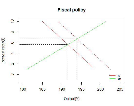 |
| Effect of fiscal policy |
An increase in the money supply by the central bank (monetary policy) results in the rightward shift in the LM curve. This happens because of the increase in nominal money supply (MS), and since the prices are exogenous the entire curve shifts to the right. Monetary policy (with exogenous prices) leads to fall in interest rates and rise in the output.
 |
| Effect of monetary policy |
Mixture of monetary and fiscal policy
Any desired level of output and interest rates can be achieved by using both these policies in tandem, as illustrated below.
 |
| Effect of both fiscal and monetary policy |
Aggregate demand curve (AD curve)
Now if we introduce prices in the picture we can trace out different combinations of “P“(prices) and “Y” for which both the goods and the money market are in equilibrium. In order to achieve this we have endogenised the computation of prices (P) (by taking ms = (nominal money)/(prices)) This represents an important relationship between aggregate price level and output for the economy. The downward sloping AD curve should not be confused with the demand curve for a good (as in microeconomics). Although both are downward sloping, the reasons for the negative relation between the prices and output demanded are different in the 2 cases. In microeconomics if the price of a good increases less of it is demanded, ceteris paribus. However in the case of AD curve, this negative relation is established by the interplay between the goods and the money market that ensures that markets clear.

This completes the story from the demand side, as to how we arrived at the aggregate demand curve for the economy. Note that we have taken a simplified version of the equations to make our point clear and to make it useful for non-econ students too. We could introduce government taxes to make the equations more realistic (and complicated) but the math looks cleaner this way and anyways the intuition remains the same even after incorporating taxes.
The next thing that we need to do is to arrive at the aggregate supply curve (labor side) for the economy, which we shall take up in the next post. Once we have presented both the ideas of aggregate demand and aggregate supply, we would be in a position to better understand the above discussion about the classical and Keynesian school of thought.
To leave a comment for the author, please follow the link and comment on their blog: We think therefore we R.
R-bloggers.com offers daily e-mail updates about R news and tutorials about learning R and many other topics. Click here if you're looking to post or find an R/data-science job.
Want to share your content on R-bloggers? click here if you have a blog, or here if you don't.