
Elements of Bayesian Econometrics
[This article was first published on Econometric Sense, and kindly contributed to R-bloggers]. (You can report issue about the content on this page here)
Want to share your content on R-bloggers? click here if you have a blog, or here if you don't.
Want to share your content on R-bloggers? click here if you have a blog, or here if you don't.

posterior = (likelihood x prior) / integrated likelihood
The combination of a prior distribution and a likelihood function is utilized to produce a posterior distribution. Incorporating information from both the prior distribution and the likelihood function leads to a reduction in variance and an improved estimator.
As n→ ∞ the likelihood centers over the true β. As a result, with more data the role of the likelihood function becomes more important in deriving the posterior distribution.
P(θ|y) = (P(y|θ)*P(θ) )/(P(y) = ( P(y|θ)*P(θ) ) / ∫ (P(y|θ)*P(θ) )/dθ
P(θ|y) = posterior distribution
P(y|θ) = likelihood function L(θ)
P(θ) = prior distribution
P(y) = ∫ (P(y|θ)*P(θ) )/dθ = the integrated likelihood, a normalizing or proportionality factor
P(θ|y) α P(y|θ)*P(θ) –> the posterior distribution is a weighted average of the prior distribution and the likelihood function
Deriving the posterior distribution may be an algebraic exercise, but summarization is more difficult, requiring numerical methods. We may often be interested in deriving the posterior expected value of θ.
E(θ|y) = ∫ θ f(θ|y) dθ
This may be approximated numerically using a sequence of random draws Θ(1) , Θ(1) , …Θ(G)
E(θ|y) = 1/G ∑ Θ(g)
This can actually be implemented via Markov Chain Monte Carlo methods. For the sequence of draws Θ(1) , Θ(1) , …Θ(G) , Θ(g+1) depends solely on the previous draw Θ(g) forming a markov chain which converges to the target density.
LOSS FUNCTIONS
Define l(Θ(hat) ,Θ) as the loss from the decision to choose Θ(hat) to estimate Θ
Ex: squared error loss l(Θ(hat) ,Θ) = (Θ(hat) – Θ)^2
choose Θ(hat) to minimize E[l(Θ(hat) ,Θ)] = ∫ l(Θ(hat) ,Θ) p(θ|y) dθ
REGRESSION ANALOGY
Recall, that if we specify the following likelihood:
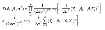
ΒOLS = BMLE = (X’X)-1X’y
If we specify a prior distribution for β as P(β) α exp[(β – m) V-1 (β – m)/2]
i.e β ~N(m,V)
and
σ2 ~ I gamma(v/2,ς/2)
Given the specified priors and likelihood, we can express the posterior distribution as:
p( β , σ2 |y) α p(y|β , σ2 ) p(β , σ2 )
Bayesian models can be implemented using the package MCMCpack in R.
An example given by Martin (one of the developers of the package) involves modeling murder as a function of unemployment.
Under the linear regression model we get the following results:
Using bayesian methods, with standard priors we get very similar results:
Bayesian methods with informative priors (as specified in the earlier discussion above)
References:
An example given by Martin (one of the developers of the package) involves modeling murder as a function of unemployment.
Under the linear regression model we get the following results:
Call:
lm(formula = murder ~ unemp, data = murder)
Residuals:
Min 1Q Median 3Q Max
-5.5386 -2.6677 -0.6324 2.3935 8.9443
Coefficients:
Estimate Std. Error t value Pr(>|t|)
(Intercept) -0.5509 2.4810 -0.222 0.82521
unemp 1.4204 0.4535 3.132 0.00296 **
—
Signif. codes: 0 ‘***’ 0.001 ‘**’ 0.01 ‘*’ 0.05 ‘.’ 0.1 ‘ ’ 1
Residual standard error: 3.599 on 48 degrees of freedom
Multiple R-squared: 0.1697, Adjusted R-squared: 0.1524
F-statistic: 9.809 on 1 and 48 DF, p-value: 0.002957
Using bayesian methods, with standard priors we get very similar results:
Iterations = 1001:11000
Thinning interval = 1
Number of chains = 1
Sample size per chain = 10000
1. Empirical mean and standard deviation for each variable,
plus standard error of the mean:
Mean SD Naive SE Time-series SE
(Intercept) -0.5278 2.5374 0.025374 0.023700
unemp 1.4158 0.4648 0.004648 0.004426
sigma2 13.5547 2.9186 0.029186 0.035616
2. Quantiles for each variable:
2.5% 25% 50% 75% 97.5%
(Intercept) -5.5103 -2.189 -0.493 1.147 4.402
unemp 0.4957 1.112 1.412 1.719 2.329
sigma2 9.0343 11.496 13.151 15.199 20.355
Bayesian methods with informative priors (as specified in the earlier discussion above)
Iterations = 1001:11000
Thinning interval = 1
Number of chains = 1
Sample size per chain = 10000
1. Empirical mean and standard deviation for each variable,
plus standard error of the mean:
Mean SD Naive SE Time-series SE
(Intercept) -0.317 0.9147 0.009147 0.008721
unemp 1.392 0.1885 0.001885 0.001908
sigma2 13.306 2.8145 0.028145 0.033750
2. Quantiles for each variable:
2.5% 25% 50% 75% 97.5%
(Intercept) -2.123 -0.925 -0.3036 0.2991 1.485
unemp 1.026 1.266 1.3907 1.5147 1.769
sigma2 8.916 11.296 12.9415 14.9085 19.802
References:
Andrew D. Martin. “Bayesian Analysis.” Prepared for The Oxford Handbook of Political Methodology. Click here for the chapter.
Andrew D. Martin. “Bayesian Inference and Computation in Political Science.” Slides from a talk given to the Department of Politics, Nuffield College, Oxford University, March 9, 2004. Click here for the slides, and here for the example R code.
An Introduction to Modern Bayesian Econometrics. Tony Lancaster. 2002. http://www.brown.edu/Courses/EC0264/book.pdf
R-Code :
#   ------------------------------------------------------------------
#  | PROGRAM NAME: EX_BAYESIAN_ECONOMETRCS
#  | DATE: 9-15-11
#  | CREATED BY: MATT BOGARD
#  | PROJECT FILE: WWW.ECONOMETRICSENSE.BLOGSPOT.COM
#  |----------------------------------------------------------------
#  | ADAPTED FROM: Andrew D. Martin. "Bayesian Inference and Computation in Political Science." Slides from a talk given to the Department of Politics, Nuffield College, Oxford University, March 9, #      |   2004.   SLIDES:http://adm.wustl.edu/media/talks/bayesslides.pdf  R-CODE :  http://adm.wustl.edu/media/talks/examples.zip
#  |
#  |
#  |
#  |------------------------------------------------------------------


setwd('/Users/wkuuser/Desktop/Briefcase/R Data Sets')

library(MCMCpack)
murder <- read.table("murder.txt", header=TRUE)
names(murder)
dim(murder)

# estimation using OLS
lm(murder ~ unemp, data=murder)
summary(lm(murder ~ unemp, data=murder))

# posterior with standard priors
post1 <- MCMCregress(murder ~ unemp, data=murder)
print(summary(post1))

# posterior with informative priors
m <- matrix(c(0,3),2,1)
V <- matrix(c(1,0,0,1),2,2)
post2 <- MCMCregress(murder ~ unemp, b0=m, B0=V, data=murder)
print(summary(post2))To leave a comment for the author, please follow the link and comment on their blog: Econometric Sense.
R-bloggers.com offers daily e-mail updates about R news and tutorials about learning R and many other topics. Click here if you're looking to post or find an R/data-science job.
Want to share your content on R-bloggers? click here if you have a blog, or here if you don't.